Nexus of certain model-based estimators in remote sensing forest inventory

1.   Introduction

To meet net-zero goals by mitigating the net release of greenhouse gases, the United Nations Framework Convention on Climate Change mandates annual estimates of biotic and abiotic variables of interest (VOIs) for monitoring emissions from the land-use, land-use change, and forestry sector (COP 21, 2015; IPCC, 2018). Additionally, the Food and Agriculture Organization of the United Nations underscores the importance of conducting forest inventories at local, regional, national, or global levels (FAO, 2024). Many countries’ National Forest Inventory (NFI) program readily offer precise estimates of this sort every five years using stratified or other probability sampling procedures, categorized as design-based inference (Tomppo et al., 2010). However, it is difficult and expensive for these programs to meet precision standards for annual reporting, as the annual sample size of observations for a VOI in, e.g., the US and China is only one fifth of the full sample size of just over 400,000 plots, despite being spatially balanced (Vidal et al., 2016; Hou et al., 2021). This small sample size problem challenges monitoring efficiency and reliability because design-based inference relies on large sample sizes for adequate precision (Cochran, 1977; Särndal et al., 1992).

Model-based inference can be a remedy for small sample size problems (Faber and Fonseca, 2014; Vandendijck et al., 2016). In comparison to design-based inference, it can offer a higher level of precision with the same sample size, or alternatively, a similar level of precision with a smaller sample size (Hou et al., 2019, 2023). Model-based inference is based on the concept of a population generated by a superpopulation model (Chambers and Clark, 2012). Conceptually it is quite different from design-based inference. The latter mode of inference asserts that the population studied is fixed, but unknown. Probability theory applies because we select random samples of population elements, based on which we infer properties of the population (Gregoire, 1998). In model-based inference, probability theory applies because the superpopulation model generates random populations; however, the population elements and associated auxiliary data remain constant under standard conditions (Graubard and Korn, 2002); it is only the VOIs for the population elements that vary. This inference paradigm does not require probability sampling for observing y and X during the model construction phase. Nevertheless, probability sampling ensures resilience against deviations from the assumed proxy superpopulation model with a sample that is balanced or representative in X (Chambers and Clark, 2012). A sample that is balanced in X is one where the sample mean of the X-values approximates the population mean of the X-values (Thompson, 2012).

Remote sensing (RS) has made it possible to conduct forest inventory through use of conventional model-based (CMB) inference. The CMB estimator can produce accurate estimates not only in a timely manner but also at various geographical scales (McRoberts et al., 2006, 2013, 2018). However, the CMB estimator necessitates remotely sensed auxiliary variables, X, available wall-to-wall, meaning available for every element of a population under consideration (Hou et al., 2018). This full RS coverage requirement poses a challenge for cost-efficient monitoring at national, provincial, or even county levels using advanced instruments such as high-resolution spectral or LiDAR sensors, and thus acts as a barrier to achieving information for pursuing net-zero objectives. Solutions need to be explored.

Hybrid estimators potentially offer feasible solutions. These estimators are compatible with non-wall-to-wall X selected using probability sampling and are considered as special instances of model-based inference (Ståhl et al., 2016). There are two distinct phases involved in Hybrid estimation. The first phase involves probability sampling of X, while model-based principles are applied to the second phase, and the two phases are independent of each other (Ståhl et al., 2011). However, while Hybrid estimation does support non-wall-to-wall X in the form of RS sample observations, these estimators are design-specific with (1) general properties and connections to the CMB estimator that merit further investigation; and (2) specific impacts of sampling design, RS cluster size, and coverage rate for non-wall-to-wall auxiliary data, that are not yet fully understood. Understanding the nexus of these factors could lead to increased precision and reduced costs in practical applications.

Consequently, our objectives are to (1) shed further light on the connections between different Hybrid estimators, and between CMB and Hybrid estimators, through analytical assessment and Monte Carlo simulations; and (2) compare the effects and explore the tradeoffs related to the sampling design, coverage rate, and RS cluster size on estimation precision.

2.   Model-based theories to support remote sensing forest inventory

2.1   Overview

Model-based estimators utilize a proxy of the superpopulation model for the relationship between the VOI and the auxiliary variables, X, to estimate or predict parameters for the real-world population, such as the population mean, μ, or total, τ, for the VOI (Hansen et al., 1983). Based on the remotely sensed X being wall-to-wall or not, there are at least two types of estimators used in model-based inference: the CMB estimator and Hybrid estimators. The CMB estimator requires wall-to-wall X, while Hybrid estimators can work with non-wall-to-wall X selected by probability sampling. This section will first introduce four model-based estimators, and then illustrate their connection and integration through transiting from sampling of auxiliary data to wall-to-wall coverage, and through estimator transformation. The analytical discoveries are empirically examined with Monte Carlo simulations in Section 3. The findings may benefit both theory and practice, facilitating broader use of model-based inference for remote sensing-assisted forest inventory.

With wall-to-wall or sample-based acquisition of X, we consider four cases, as listed in Table 1.

Table  1.  The four cases of wall-to-wall or sample-based acquisition of X.

Case A	CMB estimator for wall-to-wall X		${\hat{\mu }}_1$, $\widehat{Var}\left({\hat{\mu }}_1\right)$
Case B	Hybrid estimation for non-wall-to-wall X
	Case B.1	Simple random sampling of X	${\hat{\mu }}_2$, $\widehat{Var}\left({\hat{\mu }}_2\right)$
	Case B.2	Cluster sampling of X	${\hat{\mu }}_3$, $\widehat{Var}\left({\hat{\mu }}_3\right)$
	Case B.3	Stratified sampling of X	${\hat{\mu }}_4$, $\widehat{Var}\left({\hat{\mu }}_4\right)$

 | Show Table

DownLoad: CSV

These four model-based estimators are based on four foundational assumptions: (Ⅰ) a target population U comprises N elements; (Ⅱ) a sample S1 selected from U contains m elements, with each element having remotely sensed auxiliary variables, X, observed, except for the Hybrid estimator for cluster or stratified sampling of X where m represents the number of clusters, each containing A elements; (Ⅲ) a sample $S2$ containing $n2$ elements for which each element has both y and X observed; (Ⅳ) the sample $S2$ divides into $S2\_1$ (containing $n2\_1$ elements), $S2\_2$ (containing $n2\_2$ elements) and so on due to stratum-specific modeling in Case B.3. The cluster size is denoted by A, and the remote sensing coverage rate by the sampling intensity of $S1$, i.e., $mA/N$.

2.2   Conventional model-based estimator for wall-to-wall X

The CMB estimator utilizes a model to predict $\mu$ or $\tau$ of a VOI. Our study specifically focuses on $\mu$, because $\tau$ is then straightforwardly derived as $\tau =N\mu$. The model may be linear or nonlinear and can be expressed as the general expression, $y_i=g\left({\mathit{x}}_i,\mathit{\alpha }\right)+{\epsilon }_i$, where $y_i$ represents the VOI value in the $i^{\text{th}}$ element of the population, ${\mathit{x}}_i$ is a vector of remotely sensed auxiliary variables, $\mathit{\alpha }$ is a vector of model parameters, and ${\epsilon }_i$ is a random error.

The point estimator, ${\hat{\mu }}_1$, is simply the mean of wall-to-wall predictions using a fitted model, expressed as

where ${\mathit{x}}_{iU}$ denotes a vector of remotely sensed auxiliary variables for the $i^{\text{th}}$ element in the population U of size N, i.e., wall-to-wall X; and ${\hat{\mathit{\alpha }}}_{S2}$ is a vector of model parameters estimated using sample $S2$. Section 2.6 provides details about the modeling and estimation of model parameters.

The variance of ${\hat{\mu }}_1$ can then be obtained through Taylor series approximation. If ${\hat{\mathit{\alpha }}}_{S2}$ is reasonably accurate, we can linearize the $g(·)$ model at true $\mathit{\alpha }$, i.e., $g\left({\mathit{x}}_{iU},{\hat{\mathit{\alpha }}}_{S2}\right)\approx g\left({\mathit{x}}_{iU},\mathit{\alpha }\right)+\left({\hat{\mathit{\alpha }}}_{{S2}_1}-{\mathit{\alpha }}_1\right)g_1^{\text{'}}\left({\mathit{x}}_{iU},\mathit{\alpha }\right)+\left({\hat{\mathit{\alpha }}}_{S{2}_2}-{\mathit{\alpha }}_2\right)g_2^{\text{'}}\left({\mathit{x}}_{iU},\mathit{\alpha }\right)+\cdots +\left({\hat{\mathit{\alpha }}}_{S{2}_p}-{\mathit{\alpha }}_p\right)g_p^{\text{'}}\left({\mathit{x}}_{iU},\mathit{\alpha }\right)$, where $g_j^{\prime }\left({\mathit{x}}_{iU},\mathit{\alpha }\right)=\partial g\left({\mathit{x}}_{iU},\mathit{\alpha }\right)/\partial {\mathit{\alpha }}_j$ is a partial derivative with respect to the $j^{\text{th}}$ of p model parameters, and then use the second moment of the linearized function to approximate the variance of ${\hat{\mu }}_1$ (Ståhl et al., 2011).

Thereby, the variance estimator of ${\hat{\mu }}_1$, $\widehat{Var}\left({\hat{\mu }}_1\right)$, is derived as

where ${\widehat{Cov}}_{S2}\left({\hat{\mathit{\alpha }}}_j,{\hat{\mathit{\alpha }}}_k\right)$ is the estimated covariance matrix for ${\hat{\mathit{\alpha }}}_{S2}$ with the $S2$ sample, and ${\hat{\overline{g}}}_j^{\prime }=\frac{1}{N}{\sum }_{i=1}^N{g}_j^{\prime }\left({\mathit{x}}_{iU},{\hat{\mathit{\alpha }}}_{S2}\right)$ is the mean of the first-order partial derivatives requiring remotely sensed wall-to-wall auxiliary variables.

2.3   Hybrid estimator for simple random sampling of X

Simple random sampling is straightforward to utilize, relatively efficient for surveying both homogenous and heterogeneous populations, although it can be expensive in terms of logistics or acquisitions due to random selection of element locations (Daniel, 2011). When simple random sampling is employed to select X of size m from U, i.e., $S1$, the point estimator, ${\hat{\mu }}_2$, is expressed as (Ståhl et al., 2011)

where ${\mathit{x}}_{i1}$ represents a vector of remotely sensed auxiliary variables for the $i^{\text{th}}$ element in the sample $S1$ of size m, i.e., non-wall-to-wall X, selected by simple random sampling without replacement; and ${\hat{\mathit{\alpha }}}_{S2}$ is the same as in Section 2.2.

To derive the variance of ${\hat{\mu }}_2$, both the sampling of $S1$ and the distribution of ${\hat{\mathit{\alpha }}}_{S2}$ are considered. Since $S2$ is independent of $S1$ due to the independency of phases, ${\hat{\mathit{\alpha }}}_{S2}$ is independent of ${\mathit{x}}_{i1}$. Given that ${\hat{\mathit{\alpha }}}_{S2}$ is unbiased or approximately so, then ${\hat{\mu }}_2-{\mu }_2=\frac{1}{m}\sum _{i=1}^{m}g\left({\mathit{x}}_{i1},{\hat{\mathit{\alpha }}}_{S2}\right)-{\mu }_2=\left[\frac{1}{m}\sum _{i=1}^{m}g\left({\mathit{x}}_{i1},{\mathit{\alpha }}_{S2}\right)-{\mu }_2\right]+\frac{1}{m}\sum _{i=1}^m\left(g\left({\mathit{x}}_{i1},{\hat{\mathit{\alpha }}}_{S2}\right)-g\left({\mathit{x}}_{i1},{\mathit{\alpha }}_{S2}\right)\right)=D_1+D_2$, where $D_1$ accounts for sampling and $D_2$ for modeling. Because the two components, $D_1$ and $D_2$, are uncorrelated, the variance of ${\hat{\mu }}_2$ is the sum of each component's variance, expressed as $Var\left({\hat{\mu }}_2\right)=\frac{N-m}{N}\frac{{\sigma }_g^2}{m}+\sum _{j=1}^p\sum _{k=1}^p{Cov}_{S2}\left({\hat{\mathit{\alpha }}}_j,{\hat{\mathit{\alpha }}}_k\right)E_{S1}\left({\overline{g}}_j^{\prime }{\overline{g}}_k^{\prime }\right)\approx \frac{{\sigma }_g^2}{m}+\sum _{j=1}^p\sum _{k=1}^p{Cov}_{S2}\left({\hat{\mathit{\alpha }}}_j,{\hat{\mathit{\alpha }}}_k\right)E_{S1}\left({\overline{g}}_j^{\prime }{\overline{g}}_k^{\prime }\right)$, where ${\sigma }_g^2$ is the population variance of $g\left({\mathit{x}}_i,\mathit{\alpha }\right)$ values; ${Cov}_{S2}\left({\hat{\mathit{\alpha }}}_j,{\hat{\mathit{\alpha }}}_k\right)$ only depends on the sample of $S2$; and ${\overline{g}}_j^{\prime }=\frac{1}{m}{\sum }_{i=1}^m{g}_j^{\prime }\left({\mathit{x}}_{i1},\mathit{\alpha }\right)$. The first term of $Var\left({\hat{\mu }}_2\right)$ arises from the sampling uncertainty due to $S1$, and the second term from the model variance. The finite-population correction factor, $\left(N-m\right)/N$, decreases $Var\left({\hat{\mu }}_2\right)$, but can be disregarded for populations that are large compared to the sample size of $S1$ (Patterson et al., 2019). Elaborate derivations can be found in Ståhl et al. (2011, Appendix).

Thereby, the variance estimator of ${\hat{\mu }}_2$, $\widehat{Var}\left({\hat{\mu }}_2\right)$, is expressed as

where $s_{\hat{g}}^2$ is the $S1$ sample variance of $g\left({\mathit{x}}_{i1},{\hat{\mathit{\alpha }}}_{S2}\right)$ prediction; ${\widehat{Cov}}_{S2}\left({\hat{\mathit{\alpha }}}_j,{\hat{\mathit{\alpha }}}_k\right)$ is the same as in Section 2.2; and ${\hat{\overline{g}}}_j^{\prime }=\frac{1}{m}{\sum }_{i=1}^m{g}_j^{\prime }\left({\mathit{x}}_{i1},{\hat{\mathit{\alpha }}}_{S2}\right)$ applies to $S1$. Notably, both the sample size of $S1$ and the model may affect $\widehat{Var}\left({\hat{\mu }}_2\right)$.

2.4   Hybrid estimator for cluster sampling of X

Cluster sampling is a cost-effective and time-efficient method due to the surveying of nearby elements in a cluster. It is especially efficient for homogeneous populations but less so for heterogeneous ones. When using cluster sampling to select X in the form of m clusters by simple random sampling without replacement, and each cluster contains A elements, i.e., $S1$, the point estimator, ${\hat{\mu }}_3$, is expressed as (Ståhl et al., 2011)

where ${\hat{G}}_i=\sum _{a=1}^{A}g\left({\mathit{x}}_{ia1},{\hat{\mathit{\alpha }}}_{S2}\right)$ is the total of $g\left({\mathit{x}}_{ia1},{\hat{\mathit{\alpha }}}_{S2}\right)$ prediction for A elements in the $i^{\text{th}}$ cluster of $S1$.

Following the same logic as in Section 2.3, the variance of ${\hat{\mu }}_3$ can be derived as $Var\left({\hat{\mu }}_3\right)=\frac{1}{A^2}\frac{{\sigma }_G^2}{m}+\frac{1}{A^2}\sum _{j=1}^p\sum _{k=1}^p{Cov}_{S2}\left({\hat{\mathit{\alpha }}}_j,{\hat{\mathit{\alpha }}}_k\right)E_{S1}\left({\overline{G}}_j^{\prime }{\overline{G}}_k^{\prime }\right)$, where ${\sigma }_G^2$ is the population variance of cluster totals based on $g\left({\mathit{x}}_i,\mathit{\alpha }\right)$ values; ${\overline{G}}_j^{\prime }=\frac{1}{m}\sum _{i=1}^m{G}_i^{\prime }\left({\mathit{\alpha }}_{S2}\right)=\frac{1}{m}\sum _{i=1}^m\sum _{a=1}^A{g}_j^{\prime }\left({\mathit{x}}_{ia1},{\mathit{\alpha }}_{S2}\right)$. Likewise, the first term of $Var\left({\hat{\mu }}_3\right)$ arises from the sampling uncertainty due to $S1$, and the second term from the model variance.

Thereby, the variance estimator of ${\hat{\mu }}_3$, $\widehat{Var}\left({\hat{\mu }}_3\right)$, is expressed as

where $s_{\hat{G}}^2$ is the $S1$ sample variance of cluster totals based on $g\left({\mathit{x}}_{ia1},{\hat{\mathit{\alpha }}}_{S2}\right)$ prediction at the element level; and ${\widehat{Cov}}_{S2}\left({\hat{\mathit{\alpha }}}_j,{\hat{\mathit{\alpha }}}_k\right)$ is estimated with $S2$; and ${\hat{\overline{G}}}_j^{\prime }=\frac{1}{m}\sum _{i=1}^m\sum _{a=1}^A{g}_j^{\prime }\left({\mathit{x}}_{ia1},{\hat{\mathit{\alpha }}}_{S2}\right)$. Note that (1) ${\widehat{Cov}}_{S2}\left({\hat{\mathit{\alpha }}}_j,{\hat{\mathit{\alpha }}}_k\right)$ is consistent with Sections 2.2 and 2.3, and (2) the sample size of $S1$ and the model may affect $\widehat{Var}\left({\hat{\mu }}_3\right)$ through either or both terms.

2.5   Hybrid estimator for stratified sampling of X

Stratified sampling is an effective method for surveying diverse populations, despite being somewhat labor-intensive in terms of stratification and computation, which can lead to increased costs (Næsset et al., 2013). In this approach, population elements are grouped into distinct strata based on similarities in a discrete variable correlated with the VOI, such as classes for forest cover, land use, or terrain (Gregoire and Valentine, 2007). Each stratum contains sample elements which allow for the estimation of a stratum-wise mean using a stratum-wise estimator. These stratum-wise estimates can then be weighted and combined to estimate the population mean.

When stratified sampling is utilized to select X in the form of m clusters via simple random sampling without replacement from respective strata, and each cluster contains A elements, i.e., $S1$, the point estimator, ${\hat{\mu }}_4$, is expressed as (Ståhl et al., 2011)

where $W_h=N_h/N$ is the weight for stratum h, which is computable using a discrete variable and is used for stratification (Bechtold and Patterson, 2005); $N_h$ and $n_h$ are the numbers of population and sample elements within stratum h. ${\hat{\mu }}_h=\frac{\frac{1}{m}\sum _{i=1}^m{G}_{ih}\left({\hat{\mathit{\alpha }}}_h\right)}{\frac{1}{m}\sum _{i=1}^{m}A}$ is the mean estimator of the $h^{\text{th}}$ stratum with notations consistent with ${\hat{\mu }}_3$. $G_{ih}\left({\hat{\mathit{\alpha }}}_h\right)=\sum _{a=1}^{A}g\left(x_{ia1},{\hat{\mathit{\alpha }}}_h\right)$ is the sum of the element level $g\left(x_{ia1},{\hat{\mathit{\alpha }}}_h\right)$ model prediction for A elements of the $i^{\text{th}}$ cluster, and ${\hat{\mathit{\alpha }}}_h$ is the estimated model parameters used for stratum h. Note that this element level model can either be a global model constructed with $S2$, or a set of stratum-specific models constructed with $S2\_1$, $S2\_2$ and so forth of respective strata.

Following the same logic as in Sections 2.3 and 2.4, the variance of ${\hat{\mu }}_4$ divides into sampling and modeling components, expressed as $V\left({\hat{\mu }}_4\right)=\frac{1}{m}\sum _{h=1}^H\sum _{k=1}^H\frac{Cov\left(G_h\left({\mathit{\alpha }}_h\right)-{\mu }_{h}A,G_k\left({\mathit{\alpha }}_k\right)-{\mu }_{k}A\right)}{A^2}{W}_h{W}_k+\sum _{h=1}^H\sum _{k=1}^H\frac{W_h{W}_k}{A^2}\sum _{j1}^{P_h}\sum _{j2}^{P_k}{Cov}_{S2}\left({\hat{\mathit{\alpha }}}_{j1h},{\hat{\mathit{\alpha }}}_{j2k}\right)E_{S1}\left({\overline{G}}_{j1h}^{\prime }{\overline{G}}_{j2k}^{\prime }\right)$. Likewise, the first term of $Var\left({\hat{\mu }}_4\right)$ arises from the sampling uncertainty due to $S1$, and the second term from the model variance.

Thereby, the variance estimator of ${\hat{\mu }}_4$, $\widehat{Var}\left({\hat{\mu }}_4\right)$, is expressed as

where importantly, the cross-stratum covariance in the second term is zero if stratum-specific models are used, and non-zero if a global model is used (Ståhl et al., 2011); ${\hat{\overline{G}}}_{j1h}^{\prime }=\frac{1}{m}\sum _{i=1}^m\sum _{a=1}^A{g}_{j1h}^{\prime }\left({\mathit{x}}_{ia1h},{\hat{\mathit{\alpha }}}_h\right)$. In case stratum-specific variance is of interest, this estimator is expressed as $\widehat{Var}\left({\hat{\mu }}_h\right)=\frac{1}{A^2}\frac{\sum _{i=1}^m\left(G_{ih}\left({\hat{\mathit{\alpha }}}_h\right)-{\hat{\mu }}_{h}A\right)}{m\left(m-1\right)}+\frac{1}{A^2}\sum _{j1}^{P_h}\sum _{j2}^{P_k}{\widehat{Cov}}_{S2}\left({\hat{\mathit{\alpha }}}_{j1h},{\hat{\mathit{\alpha }}}_{j2k}\right){\hat{\overline{G}}}_{j1h}^{\prime }{\hat{\overline{G}}}_{j2h}^{\prime }$. Note that this formula considers that samples may be selected, or models may be applied, in a way so that dependencies among strata arise, as may be the case in applications where samples of RS data extend across several strata or where the same model has been applied in several or all strata.

2.6   Modeling

Both global and stratum-specific models were developed at the element level. The global model applies to Cases A and B, while the stratum-specific models only apply to Case B.3 in Table 1. With sample $S2$, the global model takes the form of ${\mathit{y}}_{S2}=g\left({\mathit{X}}_{S2};{\mathit{\alpha }}_{S2}\right)+\mathit{\epsilon }$ where $\mathit{\epsilon }~N\left(\mathbf{0},{\mathit{\Omega }}_{S2}\right)$ and ${\mathit{\alpha }}_{S2}$ denotes a vector of model parameters to be estimated. This model illustrates the connection between the dependent VOI, ${\mathit{y}}_{S2}$ (i.e., ${\mathit{y}}_{S2}={\left[y_1,y_2,\dots ,y_n\right]}^{\prime })$, and remotely sensed independent variables, ${\mathit{X}}_{S2}$ (i.e., ${\mathit{X}}_{S2}={\left[{\mathit{x}}_1^{\prime },\dots ,{\mathit{x}}_n^{\prime }\right]}^{\prime }=\left[\mathbf{1},{\mathit{x}}_1,\dots ,{\mathit{x}}_p\right]$). Similarly, stratum-specific models depict stratum-specific relationships: with sample $S2\_1$, ${\mathit{y}}_{S2\_1}=g\left({\mathit{X}}_{S2\_1};{\mathit{\alpha }}_{S2\_1}\right)+\mathit{\gamma }$ where $\mathit{\gamma }~N\left(\mathbf{0},{\mathit{\Omega }}_{S2\_1}\right)$; and with sample $S2\_2$, ${\mathit{y}}_{S2\_2}=g\left({\mathit{X}}_{S2\_2};{\mathit{\alpha }}_{S2\_2}\right)+\mathit{v}$ where $\mathit{\nu }~N\left(\mathbf{0},{\mathit{\Omega }}_{S2\_2}\right)$.

In model-based inference, these models may be linear or nonlinear, and involve different independent variables. However, for the sake of comparability and simplicity, a linear model using the same independent variables selected through “bootstrap stepAIC” procedure (Rizopoulos, 2022) was adopted: $\mathit{y}=\mathit{X}\mathit{\alpha }+\mathit{e}$, where $\mathit{\alpha }$ corresponds to ${\mathit{\alpha }}_{S2}$, ${\mathit{\alpha }}_{S2\_1}$ or ${\mathit{\alpha }}_{S2\_2}$ in the global and stratum-specific models; $\mathit{X}$ is a design matrix; $\mathit{e}~N\left(\mathbf{0},\mathit{\Omega }\right)$ with a positive definite matrix $\mathit{\Omega }$ corresponding to ${\mathit{\Omega }}_{S2}$, ${\mathit{\Omega }}_{S2\_1}$ or ${\mathit{\Omega }}_{S2\_2}$.

The vector of model parameters $\mathit{\alpha }$ was estimated with weighted least squares to accommodate heteroscedasticity (Carroll and Ruppert, 1988). It has the form $\hat{\mathit{\alpha }}={\left({\mathit{X}}^T{\hat{\mathit{\Omega }}}^{-\mathbf{1}}\mathit{X}\right)}^{-1}{\mathit{X}}^T{\hat{\mathit{\Omega }}}^{-\mathbf{1}}\mathit{y}$, where $\hat{\mathit{\Omega }}$ is a diagonal matrix with elements ${\hat{\mathit{\Omega }}}_i={\hat{\sigma }}_i^2$ estimated using a variance function fitted with a four-step procedure detailed in McRoberts et al. (2016). The variance-covariance matrix of $\mathit{\alpha }$ was estimated with a robust HCCM estimator that attenuates the effects of leverage points (Furno, 1996), $\widehat{Cov}\left(\hat{\mathit{\alpha }}\right)={\left({\mathit{X}}^T{\hat{\mathit{\Omega }}}^{-1}\mathit{X}\right)}^{-1}{\mathit{X}}^T{\hat{\mathit{\Omega }}}^{-1}diag\left[\frac{e_i^2}{{\left(1-{\mathit{x}}_i{\left({\mathit{X}}^T{\hat{\mathit{\Omega }}}^{-1}\mathit{X}\right)}^{-1}{\mathit{x}}_i^T{\hat{\mathit{\Omega }}}_i^{-1}\right)}^2}\right]{\left({\hat{\mathit{\Omega }}}^{-1}\right)}^T\mathit{X}{\left({\mathit{X}}^T{\left({\hat{\mathit{\Omega }}}^{-1}\right)}^T\mathit{X}\right)}^{-1}$, a key term inserted into Eqs. 2, 4, 6 and 8 for quantifying model variance. Dividing $e_i^2$ by ${\left(1-{\mathit{x}}_i{\left({\mathit{X}}^T{\hat{\mathit{\Omega }}}^{-1}\mathit{X}\right)}^{-1}{\mathit{x}}_i^T{\hat{\mathit{\Omega }}}_i^{-1}\right)}^2$ inflates $e_i^2$ so that the over-influence of observations with large variance is adjusted.

Despite employing the same modeling procedures, the estimates of $\hat{\mathit{\alpha }}$ and $\widehat{Cov}\left(\hat{\mathit{\alpha }}\right)$ still vary for the global and stratum-specific models, depending on whether the sample is $S2$, $S2\_1$ or $S2\_2$. The prediction accuracy of the global model was evaluated utilizing the root mean square error, $RMSE=\sqrt{\frac{1}{n2}{\sum }_{i=1}^{n2}{\left({\hat{y}}_{S{2}_i}-y_{{S2}_i}\right)}^2}$, and its relative form $RMSE\%=RMSE/{\overline{y}}_{S2}\times 100$, where ${\overline{y}}_{S2}=\frac{1}{n2}{\sum }_{i=1}^{n2}{y}_{S{2}_i}$ denotes the sample mean of field observed VOI in $S2$. Similarly, $RMSE$ and $RMSE\%$ were calculated for stratum-specific models by substituting the subscript $S2$ with $S2\_1$ or $S2\_2$, and by substituting the sample size $n2$ with $n2\_1$ or $n2\_2$.

3.   Monte Carlo simulations

3.1   Procedures

Monte Carlo simulation encompasses a wide range of computational algorithms that utilize repeated sampling to acquire numerical outcomes (Harrison, 2010). Through the law of large numbers, the fundamental idea is to employ randomness in addressing problems inherent in probability. While the specific procedures may differ, they generally involve four steps: (1) defining a population of potential inputs, (2) randomly generating inputs from a probability distribution across the population, (3) conducting a deterministic computation on the inputs, and (4) consolidating the results (Kalos and Whitlock, 2009).

In this research, we utilized Monte Carlo simulation to validate and compare CMB and Hybrid estimators. The population is introduced in Section 3.2. Remotely sensed auxiliary variables, X, were available wall-to-wall. They were used as such in the case of CMB, but as non-wall-to-wall for Hybrid estimation. Probability samples of X were selected through sampling methods such as simple random sampling, cluster sampling, and stratified sampling. The population mean and variance estimates for a specific design were calculated with corresponding $\hat{\mu }$ and $\widehat{Var}\left(\hat{\mu }\right)$. The second and third steps were iterated a thousand times to produce averaged estimates, $\overline{\hat{\mu }}$ and $\overline{\widehat{Var}}\left(\hat{\mu }\right)$, thereby approximating $E\left(\hat{\mu }\right)$ and $Var\left(\hat{\mu }\right)$, while considering the stochastic variability inherent in sampling X. However, the crucial matter is not the quantity of repetitions, but instead the stability of the estimates. In this study, the repetitions were considered adequate as the final average of estimates across replications did not vary by more than 0.005 proportionally from any of the previous 25 averages across replications (McRoberts et al., 2023).

The remote sensing coverage rate can be represented by the sampling intensity of $S1$, i.e., $\frac{mA}{N}$, and the remote sensing cluster size A. To investigate the impact of remote sensing coverage on Hybrid estimation, we analyzed seven different sampling intensities for sampling X in various designs. Namely, $S1$ containing 720, 1,440, 3,600, 7,200, 14,400, 28,800, or 120,409 elements, corresponding to sampling intensity at 0.6%, 1.2%, 3%, 6%, 12%, 24%, or 100%. Higher sampling intensities result in greater remote sensing coverage, but also lead to higher costs. With simple random sampling of X where $A=1$, m is 720, 1,440, 3,600, 7,200, 14,400, 28,800, or 120,409. With cluster sampling of X, m depends on A, e.g., $m=720/A$ at sampling intensity 0.6%.

To assess the impact of remote sensing cluster size on Hybrid estimation, we investigated six different cluster sizes, i.e., A containing 1, 2, 3, 4, 5, or 6 elements for cluster sampling of X. Larger cluster sizes make logistics easier compared to simple random sampling, especially for terrestrial laser scanning. For instance, with cluster sampling of X, the cluster size A contains 1, 2, 3, 4, 5, or 6 elements, resulting in m being 720, 360, 240, 180, 144, or 120 ​at the sampling intensity of 0.6%. Likewise, same rule about A and m applies to the stratified sampling of X.

3.2   Population and samples

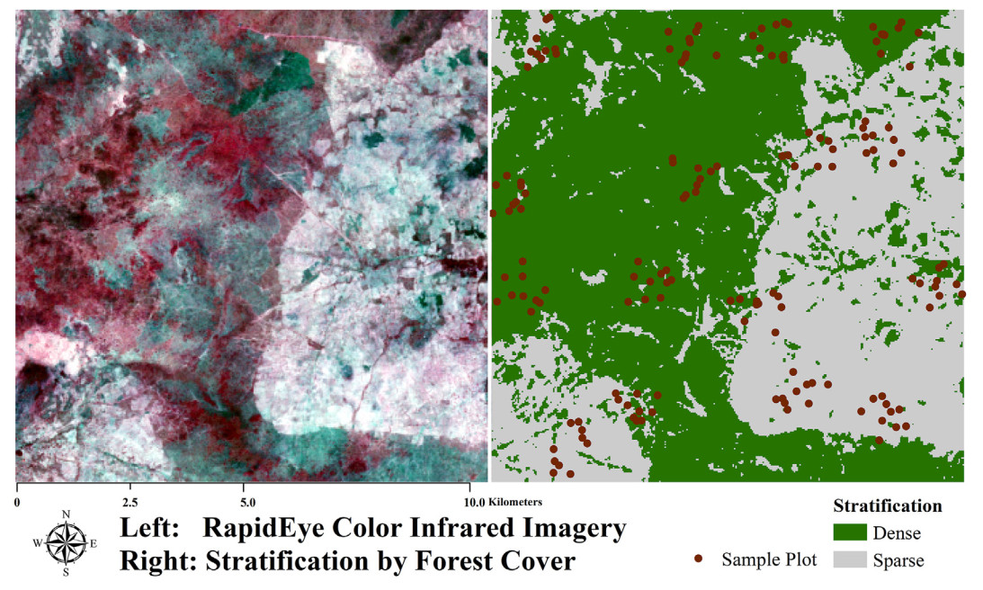
The target population sits in Kou, Burkina Faso (Fig. 1), with a population size of $N=120409$ elements, each covering an area of 30 ​m by 30 ​m. A field campaign was conducted to observe 160 sample plots between November 2013 and February 2014, following the protocols of the Land Degradation Surveillance Framework (Vågen et al., 2013). Table 2 presents the sample statistics.

Figure  1.  Target population.

DownLoad: Full-Size Img PowerPoint

Table  2.  Sample statistics.

Density attributes	Min	Max	Mean	SD
Basal area (m2·ha−1)	0	16.1	5.6	3.6
Firewood volume (m3·ha−1)	0	29.7	6.7	6.3

 | Show Table

DownLoad: CSV

The VOI represented the density of firewood volume (m³·ha⁻¹). A substantial portion of the local populace relies on subsistence agriculture and livestock farming, which are heavily dependent on the natural goods provided by trees, such as timber, firewood, medicinal plants, and animal fodder. Firewood alone accounts for approximately 90% of the total energy supply (Brännlund et al., 2009). The firewood volume in each sample plot includes both fallen and standing deadwood as well as living trees, selecting only the non-rotten, viable woody material for fuelwood. The density of firewood volume (m³·ha⁻¹) was subsequently calculated for each sample plot by dividing this plot-level firewood volume by a factor of 0.09. Due to the lack of specific allometric models for the volume of particular tree species, a generalized model for dry climates as described by Chave et al. (2005) was employed.

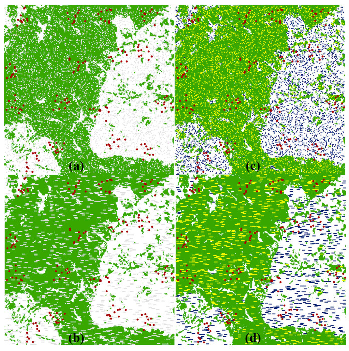
Utilizing unsupervised maximum likelihood classification (Richards, 2022), the population was categorized into dense or sparse forest cover, resulting in specific weights and samples for $S2\_1$ and $S2\_2$ (Fig. 1). The weights were 57.5% for the dense and 42.5% for the sparse forest cover areas. The sample sizes for $S2$, $S2\_1$ and $S2\_2$ in the population, dense stratum, and sparse stratum, were $n2=160$, $n2\_1=89$ and $n2\_2=71$, respectively. Fig. 2 illustrates spatial layouts for samplings X at 6% coverage. For resembling scanline patterns of ALS or UAV, a cluster consists of elements in a linear formation.

Figure  2.  Illustration of the spatial layout of $S1$ and $S2$. Subplot (a) demonstrates a simple random sample of X, subplot (b) shows cluster sampling of X, and subplots (c & d) exhibit stratified sampling of X, each at a 6% coverage rate. A cluster in subplots (b & d) includes six elements arranged linearly, mirroring scanline patterns for ALS or UAV. $S1$ comprises elements in grey in (a) and (b), and in yellow for dense stratum and blue for sparse stratum in (c) and (d); $S2$ consists of elements in red, representing sample plots from Fig. 1. (For interpretation of the references to colour in this figure legend, the reader is referred to the Web version of this article.)

DownLoad: Full-Size Img PowerPoint

3.3   Remotely sensed auxiliary variables

RapidEye imagery (RE) was acquired at a cost of 1.3 USD·km⁻², georeferenced to WGS84/UTM Zone 48N, and processed to Level-3A with a resampled spatial resolution of 30 ​m. Candidate independent variables used in modeling were calculated for RE, including the first principal component of the spectral bands (PCA), the textures of PCA, spectral features as detailed in Table 3 (www.indexdatabase.de), and the textures of spectral features. Texture calculations included the mean, variance, homogeneity, contrast, dissimilarity, entropy, angular second moment, and correlation (Haralick et al., 1973).

Table  3.  Spectral features obtained from RapidEye imagery.

Spectral Features	Formula
Enhanced vegetation index (EVI)	$2.5\left(NIR-R\right)/\left(NIR+6R-7.5B+1\right)$
Generalized Difference Vegetation Index (GDVI)	$\left({NIR}^2-R^2\right)/\left({NIR}^2+R^2\right)$
Normalized Difference Vegetation Index (NDVI)	$\left(NIR-R\right)/\left(NIR+R\right)$
Simple Ratio (SR)	$NIR/R$

 | Show Table

DownLoad: CSV

4.   Results and discussion

4.1   Validated nexus and integration

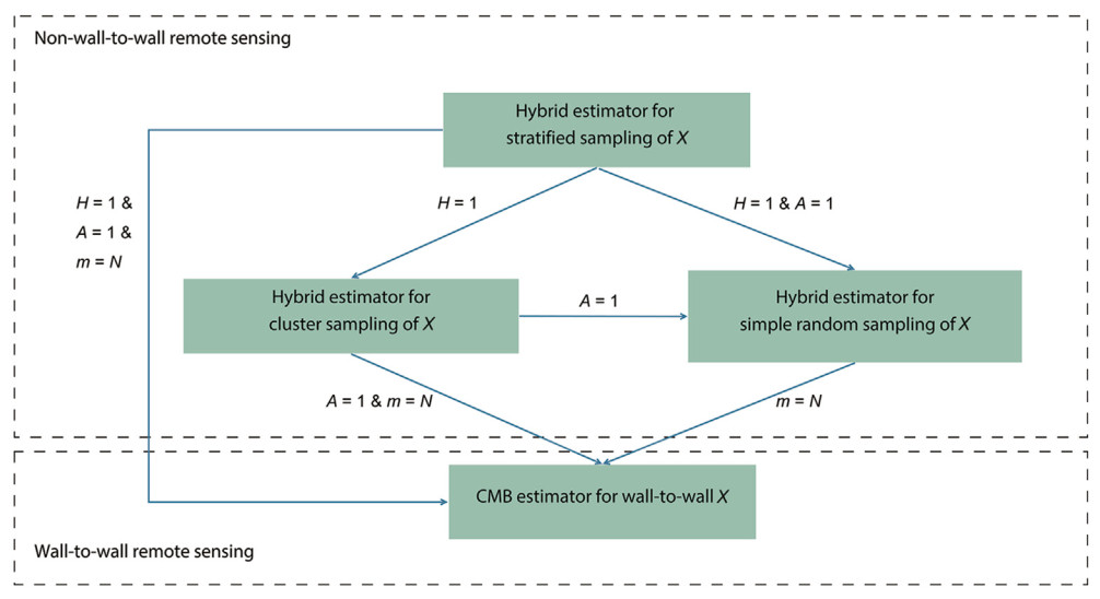
Appendix A.1 and A.2 demonstrate mathematically the connections between CMB and Hybrid estimators and the connections among Hybrid estimators. The nexus of these model-based estimators can be summarized as follows: (1) the CMB estimator for wall-to-wall X is a specific instance of the Hybrid estimator for simple random sampling of X; (2) the Hybrid estimator for simple random sampling of X is a specific instance of the Hybrid estimator for cluster sampling of X; (3) the Hybrid estimator for simple random sampling of X is a specific instance of the Hybrid estimator for stratified sampling of X; (4) the Hybrid estimator for cluster sampling of X is a specific instance of the Hybrid estimator for stratified sampling of X.

Evidently, the Hybrid estimator for stratified sampling of X is expressed in form that can be applied in multiple cases, regardless of whether the remotely sensed auxiliary variable is available wall-to-wall or non-wall-to-wall. Alternative estimators take on forms derived from this general estimator based on various sampling considerations in the acquisition of X.

Empirical results (Appendix B) of Monte Carlo simulations confirmed the analytical findings above. Fig. 3 provides an overview of these connections along with conditions outlined for equivalence. The Hybrid estimator for stratification of X represents the most general form of the scrutinized model-based estimators. Other estimators for sampling X in different ways can be derived from this general formula. Further, CMB represents a specific instance of Hybrid estimation.

Figure  3.  Nexus and integration of model-based estimators through converting the sampling of remotely sensed auxiliary variables (X) from a population of size N by the number of strata (H), the number of elements in a cluster (A), and the number of clusters (m). With simple random sampling of X, $A=1$ holds, making m collapse to the number of elements. With remote sensing, wall-to-wall coverage is expressed by $m=N$, non-wall-to-wall coverage by $m\ne N$, and the cluster size by A.

DownLoad: Full-Size Img PowerPoint

The rationale behind Fig. 3 can be applied to hierarchical model-based estimation (HMB). HMB, while not included, is a variation of CMB that breaks down the mean and variance estimators into multiple components to integrate a nested model constructed to utilize simple randomly selected, non-wall-to-wall but high-quality X (Saarela et al., 2020). The essence of HMB is to reduce CMB variance by increasing the sample size of y, not by increasing field observations, but by increasing the predicted y-values of a nested model (Saarela et al., 2022). The more accurate the predicted y-values, the more efficient the HMB estimation (Chen et al., 2023).

Based on Fig. 3, we hypothesize that a combination of Hybrid and HMB estimation can be derived to account for alternative samplings and sampling variabilities of X in the HMB process. This combination would encompass the advantages of both approaches by (1) supporting wall-to-wall mapping, (2) leveraging the strength of high-quality but non-wall-to-wall X, and (3) quantifying the uncertainty associated with sampling X (Saarela et al., 2023).

4.2   Constructed models

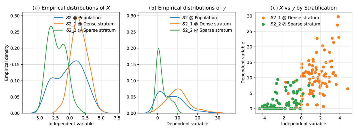
Sample balancing is associated with non-informative sampling and is a prerequisite for assuring effectiveness of model-based inference (Chambers and Clark, 2012). The samples $S2$, $S2\_1$, and $S2\_2$ were well-spread on the independent variable, PCA, of respective models in Table 4. With balanced samples, the sample means of PCA are close to the population or stratum-specific means of PCA. In our case, sample means of PCA were −0.04, 1.54 and −2.01 for $S2$, $S2\_1$, and $S2\_2$, and the population, dense stratum, and sparse stratum means, of PCA were −0.04, 1.33, and −1.89, respectively. Note that alternative classification algorithms might further improve such balancing in the respective strata (Rother et al., 2004; Silva et al., 2018). When independent variable is linearly related to y, this balancing helps to yield a more precise estimate for population parameters (Grafström and Schelin, 2014). Fig. 4 delineates covariations between dependent and independent variables at the population and stratum-levels, suggesting useful classification by forest cover.

Table  4.  Constructed global and stratum-specific models.

Model	Independent variable	$\hat{\mathit{\alpha }}$	$diag\left(\sqrt{\widehat{Cov}\left(\hat{\mathit{\alpha }}\right)}\right)$	RMSE (m3·ha–1)	RMSE%
Global ${\mathit{y}}_{S2}$	(Intercept)	6.72	0.34	4.35	64.18
	PCA	1.95	0.11
Dense ${\mathit{y}}_{S2\_1}$	(Intercept)	7.58	0.73	5.22	50.09
	PCA	1.85	0.41
Sparse ${\mathit{y}}_{S2\_2}$	(Intercept)	4.19	0.62	2.45	111.44
	PCA	0.99	0.19
All parameter estimates were significantly different from zero at significance level 5%.

 | Show Table

DownLoad: CSV

Figure  4.  Empirical distributions for the density of firewood volume (y) and PCA (X) at the population and stratum-levels.

DownLoad: Full-Size Img PowerPoint

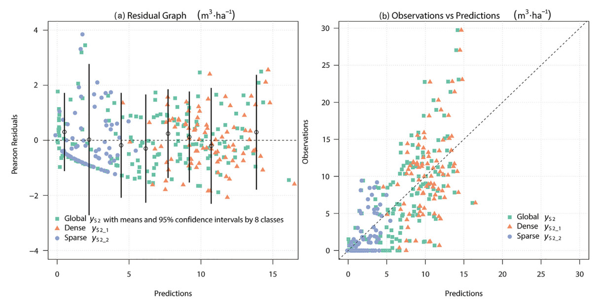
Table 4 summarizes the global model constructed with $S2$, the dense-stratum model with $S2\_1$, and the sparse-stratum model with $S2\_2$. No model exhibits any systematic lack of fit, as indicated by the absence of trends in the residual diagnostic graph, as shown in Fig. 5. The dense-stratum model has the highest prediction accuracy rank in RMSE, followed by the global model, and the sparse model. The global model was utilized across all estimators, encompassing the CMB estimator for wall-to-wall X, as well as Hybrid estimators for sample-based X. Conversely, the stratum-specific models were exclusively applied to the Hybrid estimator for stratified sampling of X.

Figure  5.  Graphs of residuals and predicted versus observed values for the different models.

DownLoad: Full-Size Img PowerPoint

4.3   Total remote sensing coverage outperformed by remote sensing sampling

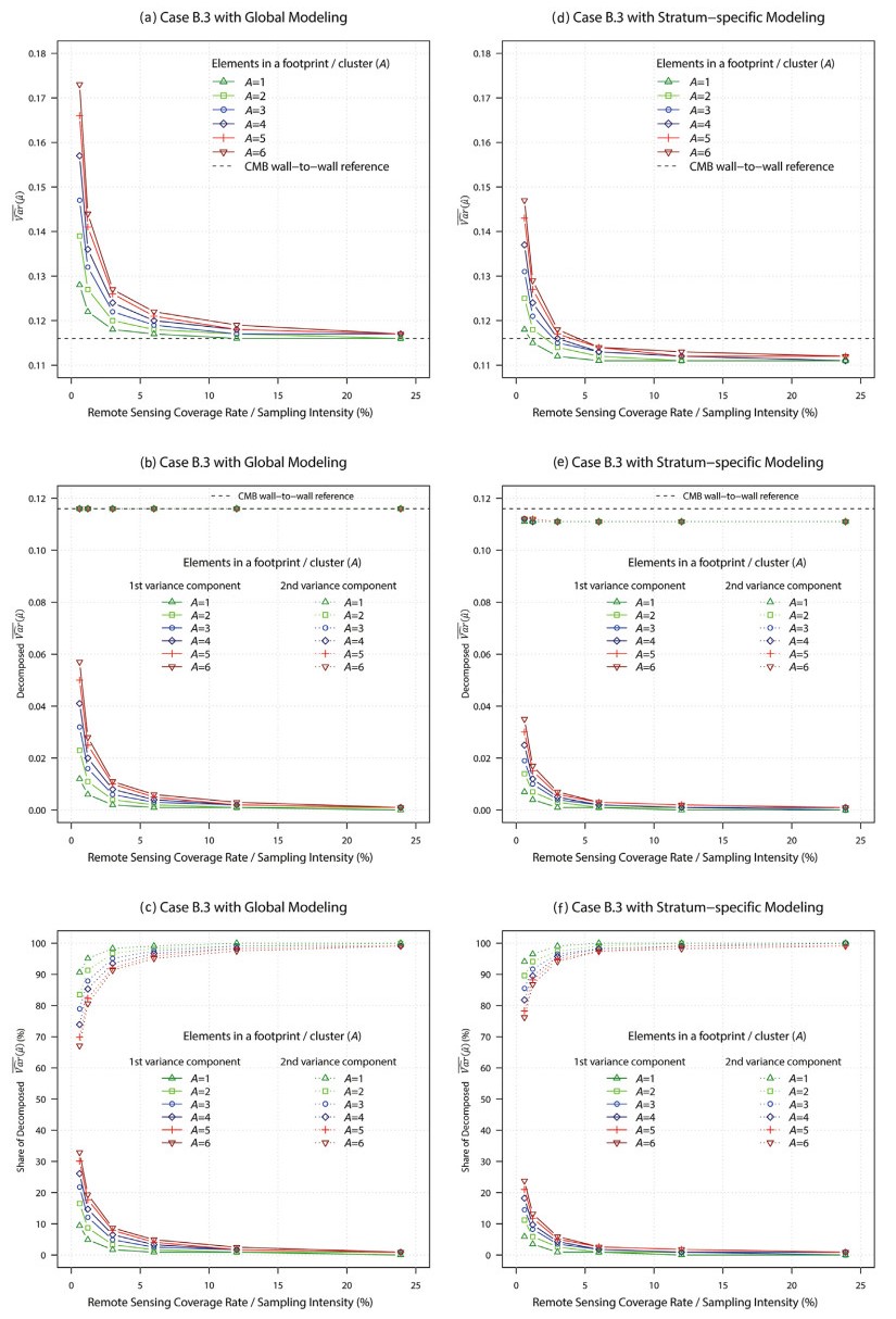
The influence of remote sensing sampling, coverage, and cluster size on inference is documented in Appendix C with generalizability discussed in Appendix D. Fig. 6 presents a summary of the results obtained from Hybrid estimation for the stratified sampling of X using global or stratum-specific modeling. The variance is decomposed for sampling and modeling components, and there are four relevant findings.

Figure  6.  Hybrid estimation for stratified sampling of X using global or stratum-specific modeling based on Appendix B.

DownLoad: Full-Size Img PowerPoint

First, using stratified sampling for X can be more efficient than conducting a complete survey of X. The Hybrid estimator for stratified sampling of X, incorporating stratum-specific modeling at 6% coverage, started to demonstrate higher precision compared to the CMB estimator at 100% coverage (Fig. 6d). The variance of the Hybrid estimator with stratum-specific modeling is not only smaller than its counterpart using a global model, but it was also smaller than that of the CMB estimator with full RS coverage (Fig. 6d, e, f; Appendix). However, the main reason is not that stratum-specific models are significantly superior to the global model. As shown in Table 4, the sparse-stratum model performed twice as poorly as the global model. Both the omission of cross-stratum covariances and the stratum-specific weighting contribute to this finding. The cross-stratum covariance in the second term of Eq. 8 is zero when stratum-specific models are used and non-zero when a global model is applied. This discovery suggests a new perspective on remote sensing instrument, acquisition, and cost for planning remote sensing-assisted forest inventories. For instance, when considering the cost of planning extensive area monitoring, it may be more beneficial to obtain non-wall-to-wall UAV or LiDAR samples through stratified sampling, instead of acquiring wall-to-wall RS data for the entire population with average quality.

Second, large-scale forest inventory may not necessarily require extensive RS coverage. As the RS coverage rate increases, the sampling variance X converges to zero in a reverse J-shaped pattern, with cost-effective sample size in our case at 12%, indicating little need for wall-to-wall coverage of X (Fig. 6a, b, c; Appendix); the variance of the Hybrid estimator with a global model converges to the variance of the CMB estimator, consistent with the analytical finding that the CMB estimator is a special case of Hybrid estimation when applying wall-to-wall coverage. The optimal sample size of X resides at the turning point of this reverse J-shaped curve, which is, however, affected by the RS cluster size. For a given RS coverage rate, small cluster sizes are preferred. The larger the cluster size, the lower the precision, a pattern particularly noticeable at low coverages. In this study, we only discuss the scenario where the cluster sizes are equal. For cases where the cluster sizes are unequal, we refer to Ståhl et al. (2011). In general, both the CMB estimator and wall-to-wall coverage can be effectively replaced with Hybrid estimation and non-wall-to-wall coverage, which will reduce costs and improve the versatility of using cutting-edge remote sensing instruments for forest inventory. A similar remark was made for the HMB estimator in Chen et al. (2023). That said, we recognize that wall-to-wall coverage may still be required for other objectives such as cartography.

Third, the variance component of modeling, rather than sampling X, dominates the total variance. While the sampling variance decreased as the coverage rate for X increased, as expected and consistent with design-based inference (Hou et al., 2022; Xu et al., 2021), the modeling variance remained stable at a high level. This suggests that the reduction of uncertainty in modeling depends on increasing the sample size for y (i.e. the S2 sample) rather than X. Additionally, stratum-specific modeling effectively reduced both variance components. To further enhance precision, modeling is crucial by (1) increasing the sample size for y, (2) incorporating more correlated X data such as from LiDAR, (3) using stratum-specific models, and (4) refining the mathematical model form.

Fourth, the use of stratum-specific modeling offers greater flexibility and efficiency compared to global modeling. Stratum-specific modeling can result in both superior and inferior stratum-specific models relative to the global model, but it ultimately yields higher precision. This is due to the impact of good or poor models being amplified or discounted by the stratum-specific weights (Eqs. 7 and 8), leading to five implications for optimizing the sampling strategy: (1) strata with larger weights require superior stratum-specific models compared to the global model; (2) a poor stratum-specific model with a smaller weight may not significantly affect $\widehat{Var}\left(\hat{\mu }\right)$; (3) if all stratum-specific models are good, $\widehat{Var}\left(\hat{\mu }\right)$ decreases further, thereby increasing precision; (4) stratification is crucial for optimizing weights and estimation; and (5) stratum-specific modeling is versatile, allowing for the use of stratum-specific RS instruments, independent variables, and models, which enhances cost-efficiency, the reuse of existing models, and most importantly, the incorporation of county-wise models into the estimation of province-wise parameters where a county is a domain or stratum of a province in NFI programs (Czaplewski, 2023).

In the context of stratification, either independence or correlation between strata is propagated through modeling. A stratum-specific model maintains independence without the necessity to combine cross-stratum covariances. Conversely, when a global model applies to each stratum, these strata become correlated due to shared model structure and parameters, necessitating the aggregation of cross-stratum covariances. This aggregation is represented in the double summation of the second term in Eq. 8. This above is the feature of the Hybrid estimator for stratified sampling of X, rather than a feature stemming from model selection.

5.   Conclusions

The study presents eight key findings: (1) the CMB estimator for wall-to-wall X is a specific instance of the Hybrid estimator for simple random sampling of X; (2) the Hybrid estimator for simple random sampling of X is a specific instance of the Hybrid estimator for cluster sampling of X; (3) the Hybrid estimator for simple random sampling of X is a specific instance of the Hybrid estimator for stratified sampling of X; (4) the Hybrid estimator for cluster sampling of X is a specific instance of the Hybrid estimator for stratified sampling of X; (5) for a given RS coverage rate, the larger the RS cluster size the lower the precision, a pattern particularly noticeable at small RS coverage rates, indicating that a small cluster size is preferred; (6) as RS coverage rate increases, the variance of Hybrid estimators converges to that of the CMB estimator in a reverse J-shaped pattern, with cost-effective sample size in our case at about 12%, indicating little need for wall-to-wall X; and (7) an interesting observation was that the Hybrid estimator for stratified sampling of X, with stratum-specific modeling, already at 6% coverage began to show higher precisions than the CMB estimator at 100% coverage, suggesting that non-wall-to-wall but stratified sampling outperformed wall-to-wall acquisition; (8) the variance component due to modeling dominated the overall uncertainty, implying that increasing the sample size of y, using advanced X such as LiDAR, and employing alternative model forms or modeling techniques are worthy directions to explore for variance reduction. Overall, Hybrid estimation strikes a balance between cost-efficiency and flexibility for large-scale monitoring based on remote sensing data.

Data availability

Data are available on request from the authors.

CRediT authorship contribution statement

Yan Zheng: Writing – review & editing, Writing – original draft, Software, Formal analysis, Data curation, Conceptualization. Zhengyang Hou: Writing – review & editing, Writing – original draft, Validation, Supervision, Software, Resources, Project administration, Methodology, Investigation, Funding acquisition, Formal analysis, Data curation, Conceptualization. Göran Ståhl: Writing – review & editing, Writing – original draft, Validation, Methodology, Investigation, Formal analysis. Ronald E. McRoberts: Writing – review & editing, Writing – original draft, Validation, Methodology, Investigation, Formal analysis. Weisheng Zeng: Writing – review & editing, Writing – original draft, Validation, Investigation, Formal analysis. Erik Næsset: Writing – original draft, Validation, Investigation, Formal analysis. Terje Gobakken: Writing – original draft, Validation, Investigation, Formal analysis. Bo Li: Writing – original draft, Validation, Investigation, Formal analysis. Qing Xu: Writing – review & editing, Writing – original draft, Resources, Methodology, Investigation, Funding acquisition, Formal analysis, Conceptualization.

Declaration of competing interest

The authors declare that they have no known competing financial interests or personal relationships that could have appeared to influence the work reported in this paper.

Acknowledgements

We express our gratitude to Dr. Janne Heiskanen from the University of Helsinki and the Building Biocarbon and Rural Development in West Africa (BIODEV) project for managing and supporting the fieldwork in Burkina Faso.

Appendix of Supplements

Supplementary data to this article can be found online at https://doi.org/10.1016/j.fecs.2024.100245.