Modelling analysis embodies drastic transition among global potential natural vegetations in face of changing climate

1.   Introduction

It is an indisputable fact that the Earth has been experiencing rapid climate warming, with a speed of 0.2 ​℃ per year over the past 40 years, compared with pre-industrial levels (IPCC, 2021). The most rapid warming has been observed at high altitudes and latitudes, such as Tibet and the polar regions (Schickhoff et al., 2015). Climate warming has significantly impacted on the physiological and biochemical processes, species composition, and community structure of vegetation, and has increasingly affected atmospheric circulation and human activities in these areas (Chen et al., 2019). However, in addition to sequestering carbon, vegetation, particularly forests can physically cool nearby areas by releasing certain cooling molecules, humidifying the air and creating clouds, which alleviates climate warming to some extent (Duveiller et al., 2021; Popkin, 2019). Vegetation, therefore, rises a key function of regulating the balance of matter, energy and information among spheres of the Earth, and provides some pivotal ecosystem services, such as oxygen, fibre, fuel and food for humanity (Bonan et al., 1992).

As a crucial reference, potential natural vegetation (PNV) is essential in comparison with real natural vegetation in degraded ecosystems. Previous studies have classified regional or global PNV and analysed the sensitivity of its pattern to meteorological factors using bioclimatic or biophysical models (Zhao et al., 2002; Yuan et al., 2011; Wang et al., 2011). However, due to the overly-complicated physio-ecological procedures and the huge computation of input data for models, these studies conducted coarse spatial simulations of global PNV and failed to achieve long-time series patterns of global PNV. This limits our understanding of the adaptive mechanisms of global PNV to past and ongoing climate change.

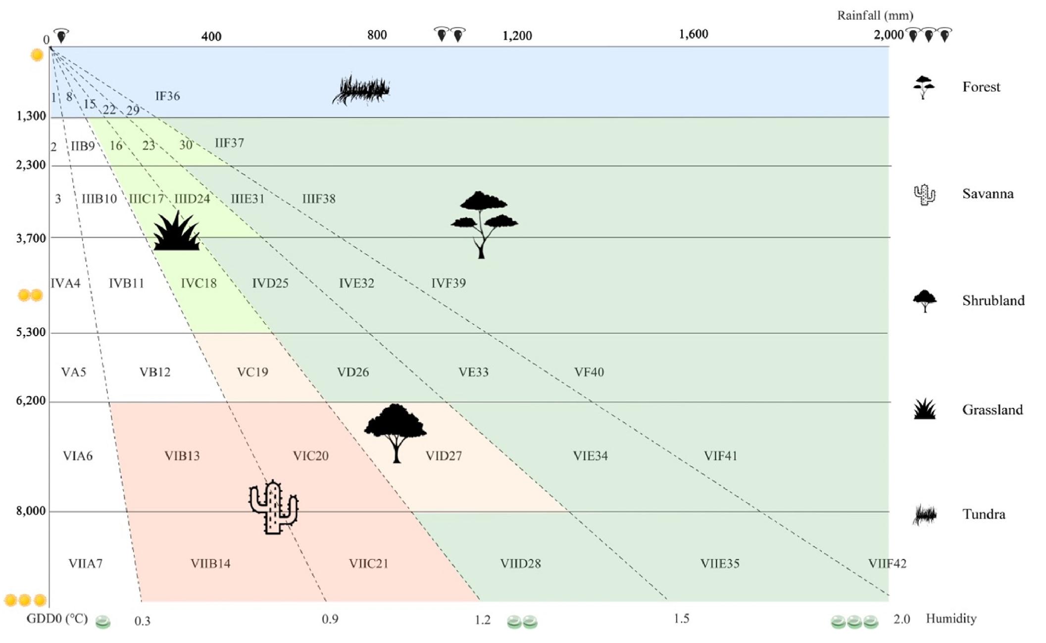
As a well-known bioclimatic model, the comprehensive and sequential classification system (CSCS) has been widely applied to classify regional or worldwide PNV (Liang et al., 2012a, 2012b; Du et al., 2021; Liu et al., 2021). The CSCS classifies PNV classes using thermal and humidity units while it calculates humidity with two stable and easily-observed meteorological variables of precipitation and temperature (Eq. 1 and Supplementary Material Table S1). 42 zonal classes of global PNV are divided by the CSCS, including desert, forest, shrubland, savanna, grassland, and tundra at the landscape level (Fig. 2; Liang et al., 2012a). Due to low consumption of time and computing resources, the CSCS is well-accepted in classifying PNV, capturing spatio-temporal distribution of PNV and predicting shift trends of PNV associated with climate change at the regional scales (Ren et al., 2021). Nevertheless, up to now, the quantitative relationship between climatic variables and PNV shift remains not well addressed.

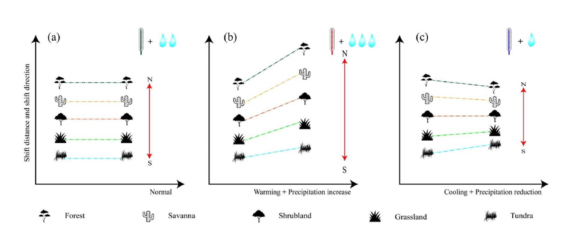
Understanding the response of PNV shifting to climate warming has recently received increased attention for a better interpretation of carbon cycling. However, accurately predicting the extent and magnitude of this shift globally using models remains challenging. For purpose of investigating the impact of climate change on variation of PNV at the global scale, we propose three hypotheses: Ⅰ. if global PNV follows the same pattern as temperature and precipitation on the Earth, the shift distance and shift direction of all five groups of global PNV would remain unchanged (Fig. 1a). Ⅱ. however, if global PNV responds to warming plus precipitation increase, some global PNV groups would be extended northward (Fig. 1b). Ⅲ. if global PNV, in contrast, responds to cooling plus precipitation reduction, some global PNV groups could be shortened toward the equator (Fig. 1c). To verify these hypotheses, this study attempts to 1) divide the detailed classes of global PNV using the CSCS and meteorological data during paleoclimatic, present and future periods; 2) visualize the spatio-temporal distribution, transition among five groups of global PNV, and analyse their responses to climate fluctuations during these periods; and 3) explore the mechanism of global PNV in face of climate change. Quantifying global PNV pattern responses to climate change at a long time-series scale helps us better understand the inherent adaption strategies of vegetation to climate change and is useful for policy decision of revegetation in damaged natural ecosystems for government.

Figure  1.  Schematic representation of climate change impacts on five groups of global potential natural vegetation under normal (a), warming plus precipitation increase (b), cooling plus precipitation reduction (c) scenarios. The thermometers with green, red and blue mercury column mean normal, warming and cooling, respectively. The numbers of sky-blue raindrop (two, three, one) represent normal, precipitation increase and precipitation reduction, respectively. The shift distance of each group for global potential natural vegetation is illustrated by the length of solid red arrows. The N and S at two endpoints of each solid red arrow indicate the direction of north and south. (For interpretation of the references to colour in this figure legend, the reader is referred to the Web version of this article.)

DownLoad: Full-Size Img PowerPoint

2.   Materials and methods

2.1   Data and pre-processing

To retrieve the paleoclimatic, historical (near current) and future spatio-temporal patterns and variations in global PNV, we downloaded three types of projected meteorological data from the global climate and weather websites (https://www.worldclim.org/data/index.html, accessed 18 October 2023). The data include monthly average minimum, maximum temperature and monthly total precipitation. The paleoclimate data was stored under version 1.4, while the historical ​and future climate data was stored under version 2.1. These data were collected for various time periods: paleogeological periods (including LIG, Last Inter-Glacial, approximately 120,000 to 140,000 years ago; LGM, Last Glacial Maximum, approximately 22,000 years ago; MH, Mid Holocene, approximately 6,000 years ago), PD (Present Day, 1970–2000), and future periods (2030, 2021–2040; 2050, 2041–2060; 2070, 2061–2080; 2090, 2081–2100). The paleoclimatic and historical meteorological data were modelled using global climate models and the meteorological data during future periods were processed using 23 global climate models and four shared socio-economic pathways (SSP126, 245, 370 and 585). These data have a spatial resolution of 30 ​s, which is approximately 1-km, and were gridded using thin plate smoothing splines with the ANUSPLIN software (version 4.4) developed by the Australian National University (Xu and Hutchinson, 2013).

In this study, we selected the paleoclimatic, historical and future meteorological datasets modelled by CCSM4 (community climate system model version 4) and MRI-ESM2-0 (meteorological research institute-earth system model version 2.0, Japan) because they have been widely used in the fields of atmospheric science, biogeochemistry and ecology (Yukimoto et al., 2019). In addition, we chose two combinations of scenarios and periods, namely SSP370_2030 and SSP585_2090, for future meteorological datasets. These scenarios represent the lowest temperature with relatively deficient precipitation (SSP370_2030) and the highest temperature with fairly abundant precipitation (SSP585_2090) projected under scenario 370 in 2030 and scenario 585 in 2090, respectively (Supplementary Material Fig. S1). According to the classification variables and approaches of the CSCS, the projected meteorological data mentioned above were utilized to calculate the annual accumulated temperature above 0 ​℃ (GDD0) and the annual total precipitation (p) using mathematical manipulations. These calculated values were then employed in simulating humidity (h).

2.2   Principle of the CSCS

The CSCS classifies PNV using two bioclimatic variables: GDD0 and h. The humidity (h) is calculated as follows (Ren et al., 2008):

where 0.1 is the adjusted coefficient. The classification of the 42 PNV classes is presented in Supplementary Material Table S1, and the specific codes and names for each of the 42 classes can be found in Supplementary Material Table S2. To illustrate the classification process, let's consider an example. If a grid cell in the humidity (h) layer has a value greater than or equal to 2.0 (unitless) and the corresponding grid cell in the GDD0 layer has a value greater than or equal to 8,000 ​℃, this grid cell would be classified as VIIF42 (tropical-perhumid rain forest).

To facilitate the visualization of the general variation trends in the global PNV, we regrouped the original 42 classes into five groups (including forest, shrubland, savanna, grassland and tundra, desert was excluded in our analysis and not shown in Fig. 2 owing to its extremely sparse vegetation cover and most of the short-life plants emerge at the occasion of rainfall events in summer, and they complete their life history in a short time). For detailed information on the regrouping foundation and approach, please refer to Supplementary Material Table S3.

Figure  2.  Index chart for determining global potential natural vegetation class in the comprehensive and sequential classification system (modified based on Feng et al., 2013). The names of 42 PNV classes were shown in Supplementary Material Table S2. The numbers of aureate sun, black raindrop and light-green dewdrop demonstrate the degree of GDD0 (above 0 ℃ during growing degree days, ℃), rainfall (mm) and humidity (non-dimension). The classes filled with light green, red, orange, grass green and blue under the five black icons express the five groups of global potential natural vegetation of forest, shrubland, savanna, grassland, tundra, respectively. (For interpretation of the references to colour in this figure legend, the reader is referred to the Web version of this article.)

DownLoad: Full-Size Img PowerPoint

2.3   Geometrical center points, shift trends of distance and direction

The geometrical center points, shift trends of distances and directions of five PNV groups were determined following Hart (1954) and Yue et al. (2011):

where t is one of the six periods; i_m(t) and s_m(t) are the patch amount and total area (km²) of mth group during t, respectively; s_mn(t) and [x_mn(t), y_mn(t)] mean the area (km²) and coordinate (longitude and latitude, degree) of geometrical center point of nth patch in mth group during t, respectively.

D_m is the shift distance (km) of mth group from t–1 to t; [x_m(t), y_n(t)] and [x_m(t–1), y_m(t–1)] state the coordinates (longitude and latitude, degree) of geometrical center points of mth group during t and t–1.

θ_m is the shift direction (angle) of mth group from t–1 to t; 90°, 180°, 270° and 360° are defined as due east, south, west and north, respectively.

2.4   Data analysis

The area and percentage calculation of transition among the five PNV groups were generated using the patch analysis embedded in Arc Toolbox. This analysis involves a pixel-by-pixel comparison to determine the changes in group composition and the corresponding areas and percentages of transition. Meanwhile, the shift distance and shift direction of the five PNV groups were calculated using raster calculator in Arc Toolbox. Furthermore, we visualized the spatio-temporal distributions and geometrical center points, transitions, and shift trends among the five groups during the six periods using ArcMap 10.8.2 (Esri Inc., 2020). Additionally, all of the mappings in this study were resampled to a 1-km spatial resolution and attached with the World_Natural_Earth projected coordinate system, along with the WGS_1984 geographic coordinate system, to ensure accurate visualization and calculation.

The figures were plotted by "plotrix" and "ggplot2" packages in R. In order to identify important factors affecting the shift distance and shift direction, six meteorological variables including monthly average maximum temperature, monthly average minimum temperature, monthly average temperature, annual accumulated temperature above 0 ​℃, monthly total precipitation and annual total precipitation were applied into the principal component analysis with "ggcorrplot", "FactoMineR" and "factoextra" packages in R. Moreover, to better understand the underlying mechanisms of fluctuating temperature and precipitation impacting on global PNV, the Spearman coefficients were determined to judge the significant degree between two above-mentioned independent and six above-involved dependent variables using "corrplot" package in R (version 4.3.1; R Core Team, 2023).

3.   Results

3.1   Spatio-temporal distribution of global potential natural vegetation

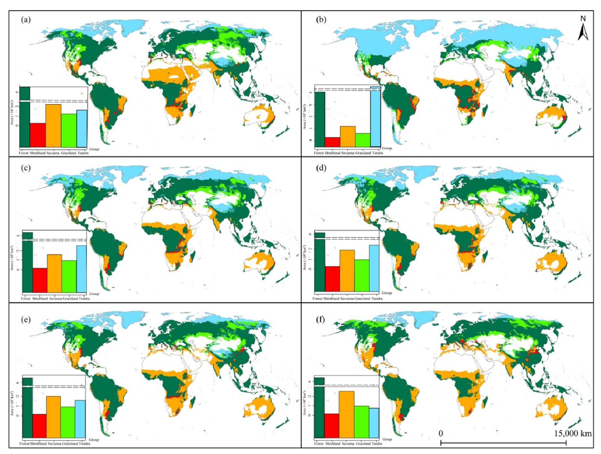
During the LIG, MH, PD, 2030 and 2090, forests exhibit the largest spatial coverage (Fig. 3a and c–f). In contrast, shrubland consistently maintains the smallest distribution potential across all six periods (Fig. 3). However, during the LGM, tundra occupies the largest extent due to the lowest temperatures and precipitation during this period. The cold and arid climate of the LGM results in the savanna and grassland also occupying a relatively small percentage of the Earth's total area (Fig. 3b). As temperature and precipitation levels rise, creating a warm-humid condition (Supplementary Material Fig. S2), thermophilic and hygrophilous plants rapidly expand their ranges, resulting in savanna and grassland surpassing the tundra in terms of spatial coverage (Fig. 3a, e and f).

Figure  3.  Spatio-temporal distributions and areas of the five groups of global potential natural vegetation during the Last Inter-Glacial (a), Last Glacial Maximum (b), Mid Holocene (c), Present Day (d), 2030 (e) and 2090 (f). Two dashed lines in each bar chart represent a y-axis break to preserve the visibility of the lowest block. The light grey lines in each sub-map mean the continental borders.

DownLoad: Full-Size Img PowerPoint

At the spatial scale, forests are predominantly distributed within the range of 30° N–60° N and 10° N–10° S, with the exception of Southeast Asia, which has a unique precipitation pattern due to the Qinghai-Tibet plateau's upheaval around 7–11 million years ago (Miao et al., 2022; Ding et al., 2022). This geographical feature, known as the 'third pole', alters the monsoon and west wind routes in Southeast Asia due to its massive mountain range. Grasslands are present briefly between 40° ​N and 60° N in the northern hemisphere. Savanna, with the broadest ecological range, stretches from 40° S to 40° N, even encompassing the majority of Australia. Shrublands are scattered in fragmented areas alongside forests, occupying the smallest total area among the five global PNV groups. Tundra is consistently found in regions with circumpolar latitudes and high elevations, such as the Arctic and the Qinghai-Tibet plateau, due to its cold and relatively humid conditions (Fig. 3). However, the spatial patterns of the five global PNV groups exhibit significant variations during the LGM and 2090, primarily due to the extremely low and high temperatures experienced during these two periods, respectively (Supplementary Material Fig. S2a and c). The exceptionally low temperatures during the LGM result in tundra expanding extensively towards equatorial latitudes, encroaching upon the niches of grasslands and forests. Consequently, the spatial extent of grasslands, forests and savannas shrinks towards the equator (Fig. 3b). Conversely, the exceptionally high temperatures in 2090 lead to the rapid retreat of tundra and the substantial expansion of forests, grasslands and savannas towards the North Pole (Fig. 3f).

3.2   Transition of global potential natural vegetation

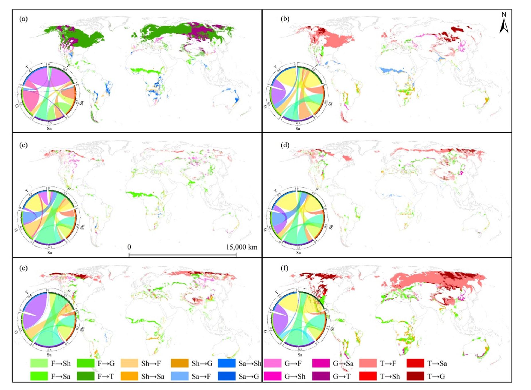
The transition from forest to tundra occurs predominantly during the phase from the LIG to the LGM, covering a vast area of 2.67 ​× ​10⁷ ​km², accounting for 87.76% of the total changed area. This conversion is more extensive compared to the transitions between the forest and the other three groups. Notably, the transformation from grassland to tundra encompasses a larger area (8.07 ​× ​10⁶ ​km²) and a higher percentage (85.34%) than the conversion occurring between grassland and the other three groups during this phase (Fig. 4a). Additionally, during the phase from the LGM to 2090, there is a significant reverse transition from tundra to forest and tundra to grassland. These conversions cover extensive areas of 2.20 ​× ​10⁷ ​km² and 8.03 ​× ​10⁶ ​km², respectively, constituting percentages of 96.34% and 90.89% (Fig. 4f). Similarly, throughout the other four transitional periods (Fig. 4b–e), interactive conversions between tundra and forest, as well as between tundra and grassland, are noticeable. This is due to the overlapping niches of plants in these three groups and their high sensitivity to fluctuations in temperature and precipitation.

Figure  4.  Quantitative and spatial transitions of the five groups for global potential natural vegetation during six distinct transitional phases: from the Last Inter-Glacial to the Last Glacial Maximum (a), from the Last Glacial Maximum to the Mid Holocene (b), from the Mid Holocene to the Present Day (c), from the Present Day to 2030 (d), from 2030 to 2090 (e) and from the Last Glacial Maximum to 2090 (f). The light grey lines in each sub-map mean the continental borders. F: Forest, Sh: Shrubland, Sa: Savanna, G: Grassland, T: Tundra.

DownLoad: Full-Size Img PowerPoint

It is indeed surprising that all noticeable transitions among groups occur in circumpolar latitudes and high elevation regions, such as the Arctic and Qinghai-Tibet plateau, which are widely recognized as ecologically fragile regions. Furthermore, it is interesting to note that no transitions have been observed between tundra and shrubland or savanna across the Earth's surface during the previous five transitional phases (Fig. 4a–e). This lack of transition is likely due to the significant geographic distances separating these three groups. However, during the phase from the LGM to 2090, an unexpected inter-conversation between tundra, shrubland and savanna is observed. This can be attributed to the substantial differences in annual mean temperature and annual precipitation, with variations of 16.07 ​℃ and 125.32 ​mm between these two periods (Supplementary Material Fig. S2). This suggests that inter-replacement among PNV groups is possible even when they are geographically isolated from each other, as long as there exists a significant hydro-thermal difference between the two periods (Fig. 4f). This explanation can be verified in the mass outbreak and extinction events caused by extreme climatic change during snowball glaciation and thermal maximum (Song et al., 2023; Stott and Kennett, 1991).

3.3   Geometrical centers, shift distances and shift directions

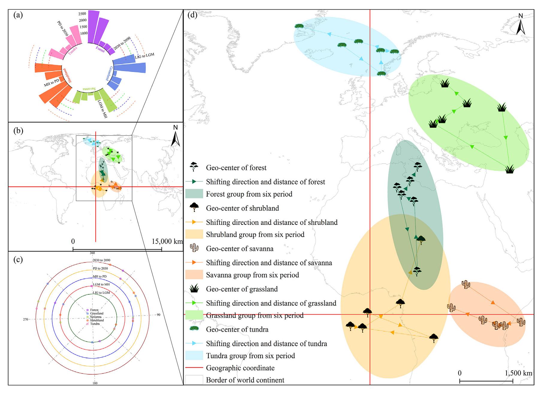
The geometrical centers of tundra are located in the Arctic region, while forest and grassland are situated in the mid-low latitudes of the northern hemisphere. Savanna and shrubland, on the other hand, are distributed near the equator. This distribution pattern generally aligns with the temperature and precipitation conditions observed during each period (Fig. 3). Over time, the savanna shifts towards northwest, while the other four groups shift northward. As the Earth becomes cooler, the geometric centers of all five groups tend to move towards more southern latitudes. It is interesting to note that even though shrubland has the smallest distribution on the Earth, it demonstrates the widest amplitude of movement among the five groups. Conversely, the savanna, despite having a larger area among the five groups, exhibits the narrowest fluctuation in its geometric center. (Fig. 5b and d).

Figure  5.  Geometrical centers (b and d, degree), shift distances (a, km), and shift directions (c, angle) of the five groups for global potential natural vegetation from the Last Inter-Glacial to 2090. The two red cross lines represent the horizontal coordinate system with the origin (0, 0). The black rectangle in the zoom-out map (b) represents the borders of the zoom-in map (d). The light grey lines in each sub-map mean the continental borders. The five black icons represent the five groups of global potential natural vegetation. (For interpretation of the references to colour in this figure legend, the reader is referred to the Web version of this article.)

DownLoad: Full-Size Img PowerPoint

As expected, the largest shift distance is observed in forest and savanna during the phase from the LIG to the LGM. This is due to the substantial temperature and precipitation differences during these two periods. However, grassland and shrubland exhibit the largest shift distance during the phase from the LGM to the MH. Meanwhile, tundra experiences the longest shift during phase from 2030 to 2090. It is noteworthy that all five groups have the shortest shift distance during the phase from the MH to the PD. This could be attributed to the relatively smaller differences in temperature and precipitation during this phase compared to that during the other five phases (Fig. 5a; Supplementary Material Fig. S2).

Surprisingly, during the phase from the LGM to the MH, tundra exhibits the largest shift direction, though previous observations indicate that forest has a slight advantage in terms of area and shift distance compared to tundra during this phase. This approximately mirrored reversal of direction for tundra and forest could potentially be attributed to the extremely low temperatures experienced during the LGM (Fig. 5c; Supplementary Material Fig. S2a and c). These extreme environmental conditions may significantly influence the shift directions of these two groups.

3.4   Global potential natural vegetation in face of climate change

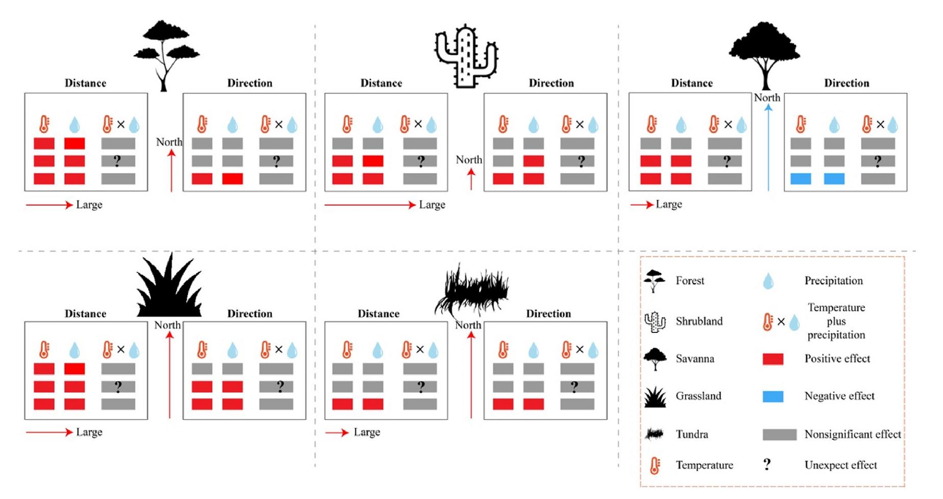
Temperature has a greater effect on the distribution, transition, shift tendency of distance and direction for five groups of global PNV than precipitation across all six periods. Principal component analysis reveals that temperature correlates positively with the shift tendency of distance and direction of global PNV, while the relationship with precipitation is negative (Supplementary Material Fig. S3a). Forest and grassland show the highest correlation (R ​≥ ​0.85) between shift distance and six meteorological factors, while tundra shows the weakest correlation (R ​ < ​0.33), with shrubland and savanna showing a moderate correlation (0.64 ​ < ​R ​ < ​0.79) (Supplementary Material Fig. S3b). The shift direction of all five groups has a lower correlation with meteorological factors compared to shift distance, with savanna displaying a negative correlation (except for GDD0, Supplementary Material Fig. S3c).

Temperature and precipitation exert the greatest effect on the shift distance of shrubland, while savanna and tundra are least affected by these two factors. With respect to shift distance, shrubland shows the weakest response to temperature and precipitation, whereas savanna, grassland and tundra exhibit the most pronounced shifts. When considering individual meteorological factors, both temperature and precipitation positively impact the shift (both distance and direction) of all five groups, except for the shift direction of savanna, which is negatively related to these two factors. Notably, both temperature and precipitation have the greatest impact on the shift distance of forest and grassland, but exert the least impact on the shift direction of forest and tundra, as well as the shift distance of tundra. At the same time, these two meteorological factors have the least relation with shift direction of forest, tundra and shift distance of tundra. Obviously, they have distinct impact on the shift direction of shrubland (Fig. 6).

Figure  6.  Mechanism schematic of the five groups for global potential natural vegetation in face of climate change. The numbers of small coloured rectangles indicate the correlation between shift distance, shift direction and metrological factors (three: high correlation; two: medium correlation; one: low correlation). The length of coloured lines with right or up arrowhead and three equidistant means the degrees between shift distance, shift direction and metrological factors (three: severe shift; two: moderate shift; one: weak shift). To further investigate the influence of climate change on shift distance and shift direction, this study employed principal component analysis in conjunction with correction tests. The principal component analysis demonstrates that temperature positively affects the shift tendency of distance and direction, while the relationship between shift distance, shift direction, and precipitation is negative (see Supplementary Material Fig. S3a).

DownLoad: Full-Size Img PowerPoint

4.   Discussion

4.1   Concept and modelling

Potential natural vegetation (PNV), initially proposed by Tüxen and Preising in 1956, refers to the hypothetical vegetation that would exist in a specific area under natural conditions, without any direct human intervention. PNV serves as a useful tool for describing the likely vegetation composition in an area and is particularly valuable for assessing regions without pristine vegetation. It assumes the absence of human activities including plowing, planting, mowing and fertilizing, etc. The CSCS utilizes two stable bioclimatic variables, namely the annual accumulated temperature above 0 ​℃ and humidity, to determine the PNV class. This classification is solely based on climatic envelope and does not consider human activities. Consequently, the vegetation classes identified by the CSCS align closely with the definition and classification of PNV, as described in detail by Ren et al. (2021).

Ecological models serve as simplified representations of ecological phenomena or processes, aiming to enhance our understanding of specific ecological patterns or processes. The focus of this study is on investigating patterns and transitions of climate-induced variations in PNV at the global scale. The study does not specifically address the verification of the effectiveness and robustness of the CSCS or conduct tests to evaluate the precision of PNV classification, which were provided in our previous study (Ren et al., 2021). While some well-known bioclimatology (Ramankutty and Foley, 1999), biogeochemistry (Holdridge, 1947) and physio-ecology process models (Smith et al., 2001) have been frequently employed for global PNV classification, the CSCS still holds significant potential due to its simplicity in terms of input/output parameters and its low time and computing requirements for large-scale vegetation classification. Moreover, the CSCS provides more numerous classifications of grassland compared to the above-mentioned models. This suggests that the CSCS, despite its simplicity, is a capable bioclimatology model suitable for large-scale classification of PNV.

4.2   Spatio-temporal distribution of global potential natural vegetation

Sun et al. (2010) conducted a study at the regional scale over centuries in the Loess Plateau in western China. Using pollen records, they found that the natural landscape during the middle Medieval Warm Period (MWP) consisted mainly of forest-rangeland. Similarly, we found that the temperate humid grassland, temperate forest and steppe emerged in the Loess Plateau during MH, resulting in a natural landscape combination of forest-rangeland. In another study, Zhang et al. (2011) examined historical documents of the late 17th century in northeast China and found that the dominant landscapes during that time were forest and grassland. In line with the historical records, we discovered that the PNV groups in northeast China consisted of steppe, temperate forest, and temperate humid grassland. These findings align with the landscapes identified in the historical records, indicating a degree of similarity between the two studies.

4.3   Global potential natural vegetation responds to climate warming

The effects of climate warming impacting on vegetation pattern are evident in various regions. As temperatures rise, tundra tends to shift northward and towards high elevations, while savanna experiences a contraction from medium latitudes towards the equator. Gonzalez et al. (2010) found that both tundra and alpine plants located in the northern hemisphere show the highest tendency to shift northward due to potential climate warming. However, the response strategies of individual plant species to projected climate warming are varied. In terms of future trends, Bakkenes et al. (2002) reviewed possible scenarios and found that by 2050, plant species would likely shift further northeast compared with their current climate envelopes. In the long term, most of the Europe potentially transitioning to a different PNV type may occur if current climate warming continues to the end of this century. Additionally, some notable change 'hotspots' include the Arctic and alpine areas, where tundra may be substituted by forest in their overlapping zone due to the sustained climate warming (Hickler et al., 2012).

Temperature seasonality is identified as the most influential predictor for vegetation distribution, followed by the annual average temperature. Among precipitation parameters, in contrast, the precipitation seasonality has the least significance in the predictive model while the annual total precipitation demonstrates a higher predictive power (Hinze et al., 2023). Overall, these findings agree with the outputs of our study, providing further support for the observed impacts of changing climate impacting on PNV distribution. They are also substantially advantageous to our understanding of the potential shifts in PNV and remarkably highlight the significance of temperature and precipitation variables in predicting vegetation responses to climate change.

4.4   Uncertainty and limiting

Our study highlights the extent, shifts and vulnerability of global PNV across different time periods, including paleogeologic eras, present day and future decades. It serves as a means to detect areas where natural vegetation may be most vulnerable to future climate warming. However, it is acknowledged that PNV, as classified by the CSCS, may differ from the actual natural vegetation that covers the Earth's surface. Moreover, PNV may be altered by other crucial factors such as topography, glacier changes, insolation, CO₂ concentrations, soil conditions and land use changes, which directly or indirectly affect the temperature and precipitation supplies to plants' survival. However, the impacts of these factors, either alone or in combination, on plant growth and vegetation dynamics have been shown to be complex, non-linear and context-dependent (Bourdouxhe et al., 2023; Liu and Yin, 2013; Sykes et al., 1999). For example, a recent study in West Africa has shown that long-term drought can cause drier tropic forests to shift towards forest communities with decreased functional, taxonomic and phylogenetic diversity. In addition, studies have also shown that rising atmospheric CO₂ concentrations may counteract the drought effects on ecosystem structure and functioning (Aguirre-Gutiérrez et al., 2020). These raise concerns about the reliability of the bioclimatic model and the precision of PNV classification.

It should be noted that due to the complexity and variability of climate and vegetation, relying solely on current anthropic cognition and abstracted model to understand ancient and future vegetation on amount, distribution, variation and response to climate change may introduce large uncertainties and limitations. To address these issues, one possible approach could be to utilize close-to-nature data, such as pollen data or remote sensing images as proxies to reconstruct historical natural vegetation and project the future potential distribution of natural vegetation worldwide. Incorporating such data could enhance the accuracy and reliability of vegetation classification and predictions. While our study does not specifically address the practices for regenerating degraded ecosystems, such as plant species selection, the output of this study can still guide ecosystem management and conservation strategies to avoid ecosystem destruction with ongoing climate warming and precipitation alteration.

5.   Conclusions

We aim to depict the spatio-temporal patterns, inter-transitions, geographical centers, shift trends of five groups of global PNV under climate change. To investigate possible mechanisms of climate change impacting on global PNV, we utilize long-time series meteorological projected data and the widely used CSCS. We find that the distribution of the five groups of global PNV generally corresponds to their ecotopes, which serve as habitats for specific species and are primarily influenced by changing climate. Sharp fluctuations of climate can lead to significant conversions among groups of global PNV, particularly in regions with circumpolar latitudes and high elevations worldwide. Changes in climate also have a fundamental influence on the geometrical centers, shift trends of PNV groups. As supposed in schema of this study (Fig. 1), warming plus precipitation increase result in the shift of forest, grassland and savanna to be extended northward while cooling plus precipitation reduction lead to tundra expanding extensively towards the equator. In some cases, even geographically distant PNV groups can be inter-replaced if there are sufficient hydro-thermal differences among different time periods. While temperature and precipitation play a dominant role in shaping PNV, some specific PNV groups exhibit heterogeneous responses to changes in these two climatic variables, reflecting the varying adaptabilities of species to climate change. The outputs of this study can serve as a valuable benchmark for community construction in ambitious ecological restoration projects worldwide. However, it is admitted that there are large uncertainties associated with the classification of PNV by the CSCS, as the projected vegetation may differ from the actual natural vegetation in nature. To address this limitation, the study suggests incorporating multiple data sources and approaches, including both bioclimatic models and close-to-nature data (e.g., remote sensing data and pollen data), which can contribute to a more comprehensive understanding of past, present, and future vegetation dynamics and inform effective ecosystem management strategies. PNV, as a critical benchmark for degraded ecosystems, can significantly reflect the impacts of global climate change on vegetation dynamics. Moreover, in order to investigate the extent and magnitude of changing climate impacting on PNV in detail, quantitative rather than qualitative analysis between PNV shift and climate drivers should be conducted in the future research.

Availability of data

The data presented in this study are available on request from the corresponding author.

CRediT authorship contribution statement

Zhengchao Ren: Writing – original draft, Visualization, Methodology, Formal analysis, Data curation, Conceptualization. Lei Liu: Writing – review & editing, Supervision, Resources, Funding acquisition. Fang Yin: Writing – review & editing, Validation, Supervision. Xiaoni Liu: Supervision, Project administration, Conceptualization.

Declaration of competing interest

The authors declare that they have no known competing financial interests or personal relationships that could have appeared to influence the work reported in this paper.

Acknowledgements

We gratefully acknowledge the data support of the global climate and weather data center. We also thank the two anonymous reviewers and the editor for their valuable assistance.

Appendix A. Supplementary data

Supplementary data to this article can be found online at https://doi.org/10.1016/j.fecs.2024.100180.