Figure
1.
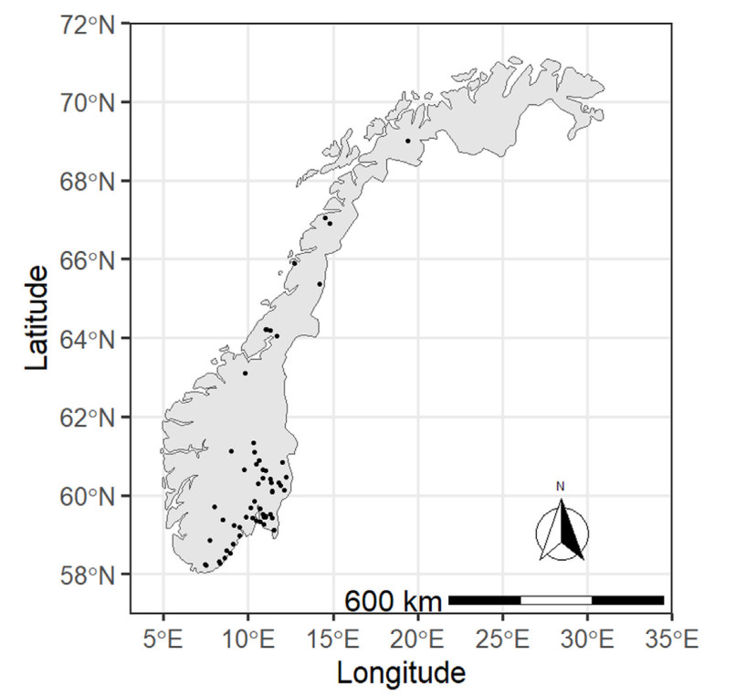
Locations of Norway spruce forest experimental sites used in this study.
| Citation: |
Christian Kuehne, Aaron R. Weiskittel, Aksel Granhus. Examining approaches for modeling individual tree growth response to thinning in Norway spruce[J]. Forest Ecosystems, 2022, 9(1): 100060. DOI: 10.1016/j.fecs.2022.100060

|
Regulating stand density through thinning is one of the most common silvicultural approaches to achieve forest management objectives (Zeide, 2001). The proper removal of trees through thinning enhances the growth and vigor of the remaining trees in the stand. Moreover, regulation of stand density through initial spacing or thinning interventions can also affect the trees' resistance towards windthrow (Gardiner et al., 1997; Achim et al., 2005). The risk of windthrow is of particular importance to shallow-rooted tree species like Norway spruce (Picea abies (L.) Karst), which in Norway is by far the commercially most important tree species, making up near one half of the growing stock by volume (Svensson et al., 2021). With a warming climate, less soil frost in winter and hence poorer root anchorage might render trees more susceptible, even if the frequency and intensity of storms do not change from the current-day situation. Yet another climate related factor to consider that comes along with warmer winters in boreal and/or mountainous regions, is the risk posed by wet snow events, which may cause extensive stem breakage and/or overturning of trees, occasionally destroying entire stands (Nykänen et al., 1997). In view of the ongoing climate change and the above-mentioned associated risks of abiotic damage, there is a need to develop density management guidelines for Norway spruce stands that can aid managers to balance production targets and stability goals.
To assess the risks of windthrow and/or snow damage in response to different spacing or thinning regimes using current mechanistic models such as e.g. HWIND (Peltola et al., 1999) and ForestGALES (Gardiner et al., 2000), information is needed on how certain stability-related tree-level variables are affected by silvicultural treatments (Gardiner et al., 2008). Important variables are amongst other tree height and a suite of other metrics that are strongly correlated with the resistance to uprooting or breakage, such as tree diameter and the height to diameter ratio. Metrics describing the size of the tree crown, such as crown volume or the ratio of crown length to total tree height, are needed as these characteristics correspond well with the wind- and/or snow-loading experienced by the trees. In turn, these metrics are largely shaped by the initial spacing and subsequent thinning(s) in the stand. While investigations of thinning in Norway spruce stands by use of long-term permanent trials have been conducted in Norway since the late 19th century (Andreassen et al., 2018), individual tree growth models which explicitly incorporate the effects of thinning, have yet to be developed for Norwegian forests (Andreassen and Tomter, 2003). The development of such models is crucial for understanding post-thinning individual tree and forest growth as well as for understanding how different stability related metrics are affected under different stand density and thinning scenarios.
Alternative approaches for modeling tree-level response to thinning have been explored (e.g. Weiskittel et al., 2011). For example, Kuehne et al. (2016) developed detailed thinning response functions for red spruce (Picea rubra Sarg.) and balsam fir (Abies balsamea [L.] Mill.) to accurately predict and quantify change in tree growth after thinning when compared to growth in trees from similar but non-thinned stands, i.e. stands of similar age, species composition, density, and site productivity (Weiskittel et al., 2011). The derived dynamic response functions in Kuehne et al. (2016) are continuous and able to exactly predict growth at any point in time after thinning mainly because of the annual resolution of the data used to build the functions. Such exhaustive data, however, is often not available given the large amount of resources necessary to collect them. Instead, permanent forest inventory or experimental plots are often monitored periodically with measurement intervals usually stretching five to ten years. Sophisticated approaches have been developed in recent years to build reliable stand- and tree-level growth and yield models based on such periodic data (McDill and Amateis, 1993; Amaro et al., 1998; Cieszewski and Bailey, 2000; Flewelling and Monserud, 2002). Among them, annualizing periodic observations has been proven to be a reliable method for modelling individual tree growth (e.g. Weiskittel et al., 2007; Kuehne et al., 2020). However, it is questionable whether such an annualization approach is capable to detect and quantify the subtle differences in growth between trees from thinned and non-thinned stands when using periodic forest growth data with varying multi-year measurement intervals.
Consequently, this work aimed to develop individual-tree models for diameter and height increment as well as crown recession using data from periodically monitored permanent plots in thinned and non-thinned Norway spruce stands in Norway. We aimed to address three research questions, namely whether i) complex thinning response functions can be fitted to data from periodic measurements with widely varying growth intervals, ii) more simple thinning modifiers including thinning indicator variables can be used in case the approach outlined in i) does not work, and iii) complex response functions are generally necessary to reliably predict individual tree growth after thinning.
Majority of the experimental stands used in this study were distributed within and covering the natural distribution range of Norway spruce in Norway, which encompasses most of southeastern and central Norway as well as northern Norway up to approximately 66°N latitude (Fig. 1). While most trials were in stands previously dominated by Norway spruce, the trials in northern Norway north of 66°N were established in first-generation spruce stands. Climatic conditions vary in the study area with mean annual temperature ranging from approximately 0.5 ℃–7.2 ℃ and mean annual precipitation varying from slightly below 400 mm and up to 1, 800 mm (1981–2010, Meteorological Institute of Norway). The current study excluded data from the southwestern and western counties with their maritime climate (Fig. 1), as growing conditions in oceanic western Norway are considered to be very different to the rest of the country (Vestjordet, 1967; Bauger, 1995).
Data used in this study were from long-term forest management trials maintained by the Norwegian Institute of Bioeconomy Research (Andreassen et al., 2018). Majority of these silvicultural experiments was established in pure, even-aged Norway spruce stands in the early 1970s as part of a larger thinning trial network (Braastad and Tveite, 2001). These trails were initially established to examine the effects of thinning from below with focus on thinning intensity and timing of thinning on stand-level volume production in 18- to 47-year-old stands. Treatments included one to three thinnings from below with different combinations of target residual trees per hectare (TPH) of 2070, 1600, 1100, and 800 at stand dominant heights of 8, 12, 16, and 20 m. However, deviations from the original experimental design resulted in a diverse dataset covering a wide range of thinning regimes varying in number of thinning interventions, time of thinning, and thinning intensity (Supplementary Material Fig. S1). We further added measurements from experimental trials from spruce stands that were never thinned. Although the trials in non-thinned stands often were established prior 1970, we only included measurements from that year onwards. At that time, these non-thinned stands were between 12 and 111 years old. Some of the plots used here contained individual trees of species other than Norway spruce, including Scots pine (Pinus sylvestris L.), birch (Betula pendula Roth, B. pubescens Ehrh.), and goat willow (Salix caprea L.). However, Norway spruce accounted for an average of 99% of total plot basal area over all plots. Plots with excessive mortality as a result of major windstorms were only included up until the occurrence of the storm event.
The final dataset comprised a total of 116, 773 diameter increment (with 41, 870 from non-thinned and 74, 903 from thinned stands), 43, 850 height increment (13, 901 from non-thinned and 29, 949 from thinned stands), and 33, 499 (8, 141 from non-thinned and 25, 358 from thinned stands) height to crown base increment (crown recession) observations (growth intervals) from 204 permanent plots in 60 trials. The length of the studied growth intervals varied between 1 and 42 years with an average of 6 years. Measurement records for all trees comprised species, vital status (live or dead) and diameter at breast height (DBH, cm). Total tree height (HT, m) and height to crown base (HCB, m) were measured for a randomly selected subsample of all live trees during every measurement campaign with about half of all trees measured for total height on average across all plots.
HT measurements missing in the final database were imputed using a total tree height equation similar to model 6 in Temesgen et al. (2007) and a mixed-modeling approach with trial as random effect. Similarly, HCB measurements missing in the final database were imputed using an equation similar to the one in Kuehne et al. (2016). Individual tree crown ratio (CR) was then calculated as the ratio of (live) crown length (HT-HCB) and HT. Basal area in larger trees (BAL, m2·ha−1) was also computed for each individual tree (Kuehne et al., 2019). Individual tree measurements were then summarized for each plot to calculate stand-level metrics including dominant height (mean height of the 100 thickest trees·ha−1, HTDOM, m) and total basal area (BA, m2·ha−1) (Table 1). Site index (SI, m) at base age 40 years was determined using the dominant height model from Allen et al. (2020). We further calculated treatment related variables including time since thinning (TST), BA (BABEFORE, BAAFTER) and TPH before as well as after each thinning intervention (TPHBEFORE, TPHAFTER), respectively, and also quantified dominant height (HTTHIN) and stand age (AGE) at the time of thinning (AGETHIN) when plot records indicated a thinning took place. An overview of the stand- and tree-level variables for each dataset used in this work is provided in Table 1.
| Attribute | Non-thinned | Thinned | All | ||||||||||||
| Mean | SD | Min | Max | Mean | SD | Min | Max | Mean | SD | Min | Max | ||||
| ΔDBH | |||||||||||||||
| DBH (cm) | 13.30 | 5.68 | 1.00 | 43.10 | 15.81 | 6.09 | 1.50 | 44.70 | 14.91 | 6.07 | 1.00 | 44.70 | |||
| HT (m) | 12.98 | 5.27 | 1.30 | 33.60 | 13.66 | 5.06 | 1.60 | 35.10 | 13.42 | 5.15 | 1.30 | 35.10 | |||
| HCB (m) | 5.66 | 3.94 | 0 | 20.50 | 4.38 | 3.33 | 0.10 | 22.39 | 4.84 | 3.61 | 0 | 22.39 | |||
| CR (m·m−1) | 0.61 | 0.18 | 0.04 | 1.00 | 0.72 | 0.14 | 0.02 | 0.99 | 0.68 | 0.16 | 0.02 | 1.00 | |||
| BAL (m2·ha−1) | 24.44 | 15.27 | 0 | 85.64 | 16.93 | 10.95 | 0 | 63.44 | 19.62 | 13.17 | 0 | 85.64 | |||
| BA (m2·ha−1) | 39.08 | 15.57 | 2.96 | 86.58 | 28.23 | 11.40 | 6.33 | 63.82 | 32.12 | 14.05 | 2.96 | 86.58 | |||
| SI (m) | 15.57 | 4.45 | 6.64 | 28.61 | 15.45 | 2.80 | 10.10 | 21.80 | 15.49 | 3.48 | 6.64 | 28.61 | |||
| ΔHT | |||||||||||||||
| DBH (cm) | 15.01 | 6.58 | 1.00 | 43.10 | 17.95 | 6.57 | 1.50 | 44.70 | 17.02 | 6.72 | 1.00 | 44.70 | |||
| HT (m) | 13.58 | 5.76 | 1.30 | 33.60 | 14.82 | 5.23 | 1.60 | 31.70 | 14.42 | 5.43 | 1.30 | 33.60 | |||
| HCB (m) | 5.59 | 4.23 | 0.01 | 20.50 | 4.88 | 3.74 | 0.10 | 21.00 | 5.10 | 3.91 | 0.01 | 21.00 | |||
| CR (m·m−1) | 0.64 | 0.20 | 0.11 | 0.99 | 0.70 | 0.15 | 0.16 | 0.99 | 0.68 | 0.17 | 0.11 | 0.99 | |||
| BAL (m2·ha−1) | 20.34 | 16.33 | 0 | 85.64 | 15.24 | 12.12 | 0 | 63.44 | 16.85 | 13.80 | 0 | 85.64 | |||
| BA (m2·ha−1) | 39.11 | 16.64 | 2.96 | 86.58 | 30.12 | 11.37 | 6.33 | 63.82 | 32.97 | 13.91 | 2.96 | 86.58 | |||
| SI (m) | 15.91 | 4.08 | 6.64 | 28.61 | 15.54 | 2.88 | 10.10 | 21.80 | 15.66 | 3.31 | 6.64 | 28.61 | |||
| ΔHCB | |||||||||||||||
| DBH (cm) | 16.08 | 6.53 | 2.30 | 43.10 | 18.28 | 6.43 | 2.40 | 44.70 | 17.75 | 6.52 | 2.30 | 44.70 | |||
| HT (m) | 14.63 | 5.60 | 2.30 | 32.00 | 15.11 | 5.06 | 2.20 | 31.70 | 14.99 | 5.20 | 2.20 | 32.00 | |||
| HCB (m) | 6.45 | 4.05 | 0.10 | 20.50 | 5.08 | 3.68 | 0.10 | 21.00 | 5.41 | 3.82 | 0.10 | 21.00 | |||
| CR (m·m−1) | 0.59 | 0.17 | 0.11 | 0.99 | 0.69 | 0.15 | 0.16 | 0.99 | 0.67 | 0.16 | 0.11 | 0.99 | |||
| BAL (m2·ha−1) | 22.40 | 17.05 | 0 | 74.74 | 15.58 | 12.00 | 0 | 63.44 | 17.24 | 13.72 | 0 | 74.74 | |||
| BA (m2·ha−1) | 44.12 | 14.26 | 10.52 | 74.99 | 30.78 | 10.66 | 8.48 | 63.82 | 34.02 | 12.97 | 8.48 | 74.99 | |||
| SI (m) | 14.94 | 4.55 | 6.64 | 23.27 | 15.31 | 2.96 | 10.10 | 21.80 | 15.22 | 3.42 | 6.64 | 23.27 | |||
 DownLoad:
CSV
DownLoad:
CSV
We started our analysis following the approach outlined in Kuehne et al. (2016). First, a baseline model (ƒBASE) not specifically accounting for thinning, i.e. not including treatment related variables was developed for all three studied response variables, i.e. annual diameter increment (ΔDBH), annual height increment (ΔHT), and annual height to crown base increment (ΔHCB). Using all observations, i.e. measurements from thinned and non-thinned stands, the following general model form was used to derive the sought-after ƒBASE equations:
| Y=exp(Xβ) | (1) |
where Y is the response variable (ΔDBH, ΔHT, or ΔHCB), Xβ is the model-specific explanatory variable design matrix (linear predictor; Zuur et al., 2009) with the associated estimated fixed (βij) and trial-specific random parameters (bij) for equation i and explanatory variable j. Random effects and residuals of the derived models were assumed to be normally distributed. Explanatory variables of Xβ comprised the previously described tree- and stand-level attributes which were added to each model in a stepwise manner depending on significance and biological plausibility.
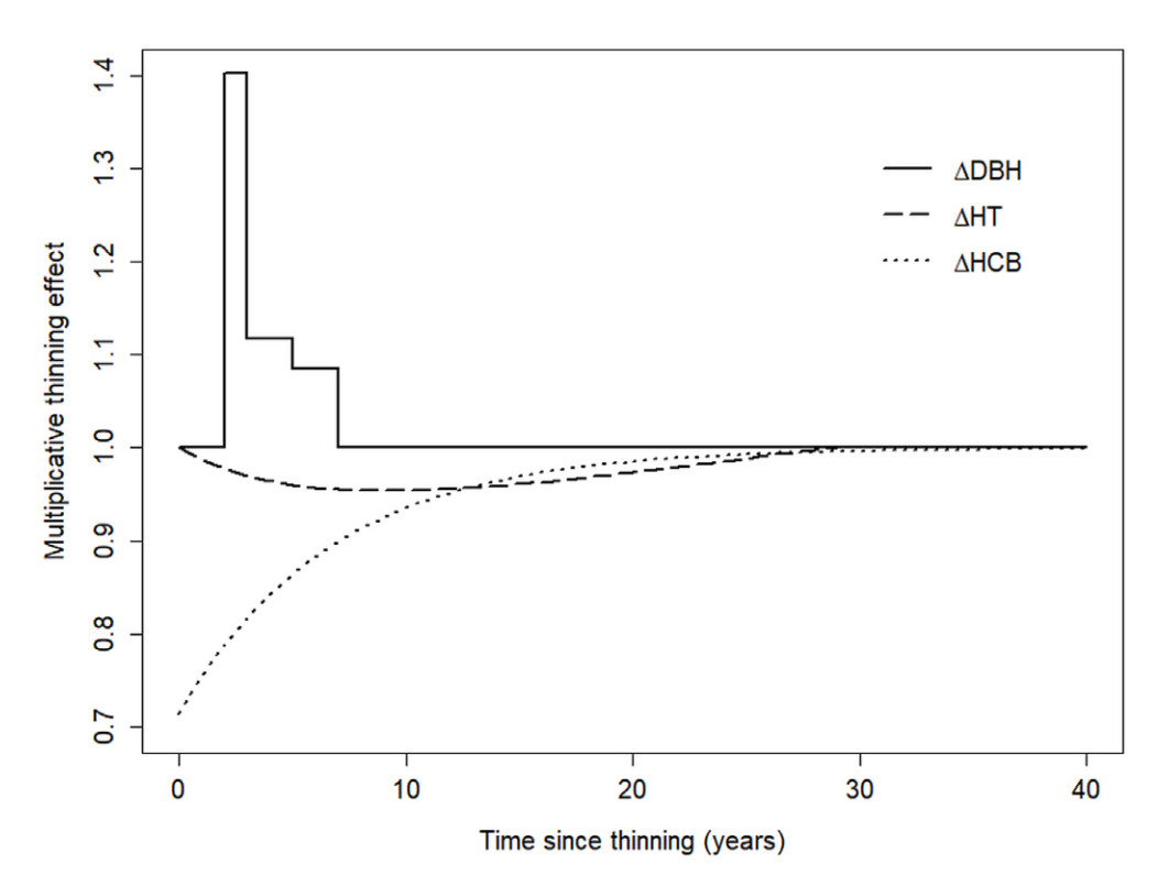
Next, we aimed to fit multiplicative thinning modifiers (ƒTHIN) following a Type 1 response as described in Snowdon (2002). Also called treatment response functions, ƒTHIN modify the outcome of ƒBASE (i.e. ƒBASE × ƒTHIN or ƒBASE + ƒTHIN for additive modifiers; Weiskittel et al., (2011) based on treatment variables with time since thinning (TST) as the most influential one. A Type 1 thinning modifier should predict a relatively rapid increase and often early maximum of the thinning effect shortly after the thinning followed by a more gradual lessening of the response over time after thinning until the thinning effect eventually diminishes and becomes zero again. The thinning effect is supposed to be positive for ΔDBH and potentially negative for ΔHT and ΔHCB (Kuehne et al., 2016). To correspond with the general response pattern for thinning interventions, we used a Type I combined exponential - power function of the following form:
| fTHIN=1±(γ21×γTST22×TSTγ23) | (2) |
where γi are fixed effect parameters and TST = 0 for non-thinned plots. To account for thinning intensity, Eq. 2 can be extended by incorporating e.g. the ratio of BAREM and BABEFORE (Kuehne et al., 2016):
| fTHIN=1±[exp(γ30+γ31100×(BAREMBABEFORE)+0.01)×γTST32×TSTγ33] | (3) |
We further examined other multiplicative modifiers including a slight modification of Eq. 5 in Gyawali and Burkhart (2015):
| fTHIN={1,TST>γ41(1BAAFTER/BABEFORE)γ40×(−(TST2)+γ41×TST)(AGETHIN+TST)2,0<TST≤γ41 | (4) |
The response predicted in Eq. 4 roughly follows the one outlined for Eq. 2 but depicts a more gradual initial increase and also needs to be restrained according to the duration parameter γ41 derived during the fitting process (Liu et al., 1995).
In contrast to Eqs. 2-4, the multiplicative thinning modifier by Hann et al. (2003) predicts a continuous, exponential treatment effect approaching 1 with increasing TST after a maximum response right after the thinning intervention:
| fTHIN=1±[γ50×(BAREMBABEFORE)γ51×exp(−γ52×TST)] | (5) |
Similarly, the modifier by Short and Burkhart (1992) follows the same exponential response trajectory:
| fTHIN=(BAAFTERBABEFORE)(γ61×(AGETHINAGE)) | (6) |
If complex modifiers as in Eqs. 2-6 could not be fitted in a biologically plausible manner and/or estimated parameters γi signaling insignificance, we tested whether TST could be fitted into ƒBASE by iteratively adding indicator variables representing varying time periods after treatment with e.g. TST2 indicating the second year after thinning and TST3‒5 representing years three to five after thinning (Bianchi et al., 2022). Final models including a thinning modifier or TST indicator variables are referred to full models (ƒFULL) hereafter.
All models were derived using nonlinear mixed effects modelling and the package 'nlme' (Pinheiro et al., 2021) of the statistical computing software R (version 4.1.2, R Development Core Team, 2021). A variance structure was incorporated to account for the variability in the most influential explanatory variable of each equation (DBH, HT, and CR for ΔDBH, ΔHT, and ΔHCB, respectively). To overcome problems of the varying measurement intervals observed in our datasets, parameters were annualized using an iterative mixed-effects technique of Weiskittel et al. (2007). Based on Cao (2000), the right side of the equation was a function that summed the predicted annualized ΔDBH, ΔHT or ΔHCB estimates, respectively, over the number of growing seasons during the observed growth period using the updated parameter estimates from the optimization algorithms. For each growing season during the growth period, DBH, HT or HCB, respectively, was subsequently updated using the annual increment estimates, while all other explanatory variables were linearly interpolated between their beginning values and ending values. SI, however, was assumed to be constant over time.
We calculated mean error (ME), mean absolute error (MAE), and relative MAE (MAE%) to evaluate and compare model prediction accuracy:
| ME=∑ni=1(yi−ˆyi)n | (7a) |
| MAE=∑ni=1(|yi−ˆyi|)n | (7b) |
| MAE%=∑ni=1((|yi−ˆyi|)yi×100)n | (7c) |
where yi is the observed DBH, HT, or HCB at the end of the measurement period, respectively, ˆyi is the predicted DBH, HT, or HCB, respectively, and n is the number of observations.
Besides DBH, the final ΔDBH ƒBASE also included CR, BA, BAL, and SI as explanatory variables. Fitting complex thinning modifier as in Eqs. 2-4 did not result in biologically plausible outcomes, while a modifier following Eq. 5 produced reasonable results (data not shown). However, incorporating indicator variables representing the third year, years four and five as well as six and seven after thinning, respectively, were significant and improved model performance. Extending these thinning indicator variables to account for thinning intensity by multiplying the ratio of BAREM and BABEFORE further improved prediction accuracy and resulted in the following best performing ƒFULL (Table 2, Fig. 2):
| Parameter | ƒBASE | ƒFULL | |||||||
| Estimate | SE | t-value | p-value | Estimate | SE | t-value | p-value | ||
| β80 | ‒5.047643 | 0.10520 | ‒47.98 | < 0.0001 | ‒5.468100 | 0.10565 | ‒51.76 | < 0.0001 | |
| β81 | ‒0.039723 | 0.00379 | ‒10.47 | < 0.0001 | ‒0.038439 | 0.00392 | ‒9.80 | < 0.0001 | |
| β82 | 0.875792 | 0.01267 | 69.12 | < 0.0001 | 0.778875 | 0.01286 | 60.55 | < 0.0001 | |
| β83 | 0.903008 | 0.01660 | 54.39 | < 0.0001 | 1.023460 | 0.01678 | 60.98 | < 0.0001 | |
| β84 | ‒0.000668 | 0.00001 | ‒137.06 | < 0.0001 | ‒0.000695 | 0.00001 | ‒139.51 | < 0.0001 | |
| β85 | ‒0.308305 | 0.00733 | ‒42.05 | < 0.0001 | ‒0.122793 | 0.00851 | ‒14.43 | < 0.0001 | |
| β86 | 1.028367 | 0.01953 | 52.67 | < 0.0001 | 0.999885 | 0.01944 | 51.43 | < 0.0001 | |
| β87 | 1.692007 | 0.05448 | 31.06 | < 0.0001 | |||||
| β88 | 0.555523 | 0.06355 | 8.74 | < 0.0001 | |||||
| β89 | 0.405501 | 0.05523 | 7.34 | < 0.0001 | |||||
DownLoad:
CSV
| ΔDBH=exp ((β80+b80)+(β81+b81)×DBH+β82×ln(DBH)+β83×CR+β84×BAL2+β85×ln(BA)+β86×ln(SI)+β87×(TST3×(BAREMBABEFORE))+β88×(TST4−5×(BAREMBABEFORE))+β89×(TST6−7×(BAREMBABEFORE))) | (8) |
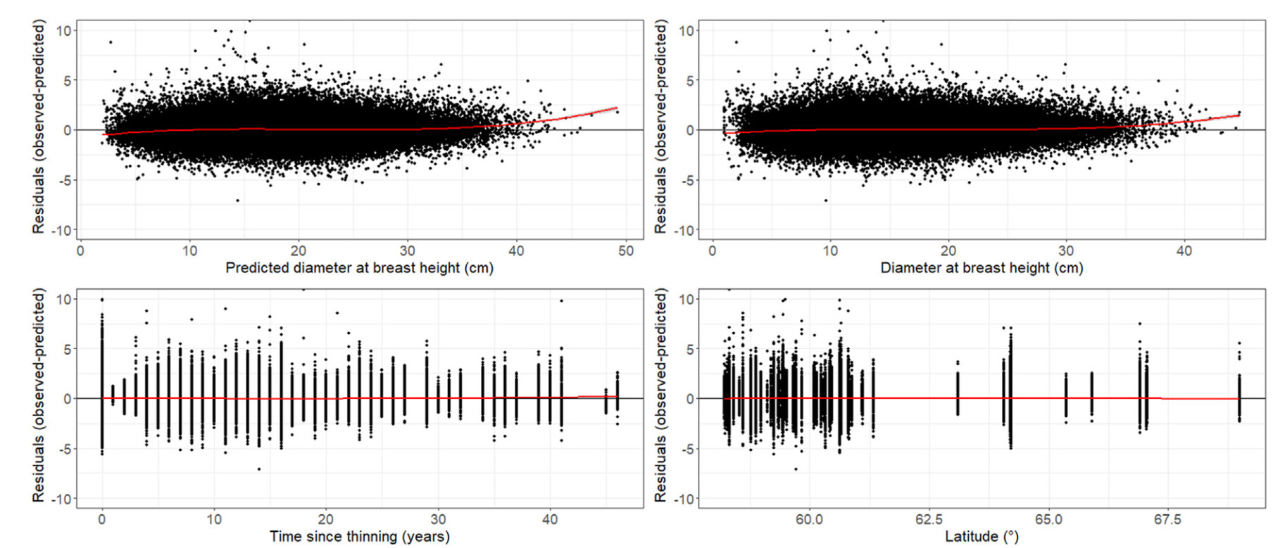
While adding the thinning indicator variables slightly improved prediction accuracy overall and for observations from thinned stands (Table 3), we found no obvious bias when plotting the residuals of ΔDBH ƒBASE (Supplementary Material Fig. S2) and ΔDBH ƒFULL over the explanatory variables including TST or other potentially influential factors such as age, elevation, and latitude (Fig. 3).
| Variable | ƒBASE | ƒFULL | |||||
| Non-thinned | Thinned | All | Non-thinned | Thinned | All | ||
| ME | ‒0.0013 | 0.0029 | 0.0014 | 0.0201 | ‒0.0082 | 0.0020 | |
| MAE | 0.4310 | 0.5332 | 0.4965 | 0.4319 | 0.5270 | 0.4929 | |
| MAE% | 3.2616 | 3.2330 | 3.2432 | 3.2746 | 3.1966 | 3.2246 | |
DownLoad:
CSV
Besides HT, the final ΔHT ƒBASE also included CR, BAL, and SI as explanatory variables. Adding a thinning effect to ƒBASE resulted in mixed and contradicting results with indicator variables representing varying time periods after thinning often suggesting a slight increase in height increment after thinning (data not shown). Fitting a response function following Eq. 5 resulted in a predicted limited negative thinning effect lasting over 50 years (data not shown). The best performing plausible ƒFULL included a multiplicative modifier following Eq. 4 predicting a marginal decrease in height increment for a time period of approximately 30 years following thinning (Table 4 and 5, Fig. 2):
| Parameter | ƒBASE | ƒFULL | |||||||
| Estimate | SE | t-value | p-value | Estimate | SE | t-value | p-value | ||
| β90 | ‒3.817176 | 0.13148 | ‒29.03 | < 0.0001 | ‒3.899612 | 0.13273 | ‒29.38 | < 0.0001 | |
| β91 | ‒0.034339 | 0.00437 | ‒7.85 | < 0.0001 | ‒0.037829 | 0.00445 | ‒8.50 | < 0.0001 | |
| β92 | 0.629971 | 0.02395 | 26.31 | < 0.0001 | 0.685842 | 0.02473 | 27.74 | < 0.0001 | |
| β93 | 0.546126 | 0.02114 | 25.84 | < 0.0001 | 0.584605 | 0.02139 | 27.33 | < 0.0001 | |
| β94 | ‒0.000365 | 0.00003 | ‒12.05 | < 0.0001 | ‒0.000358 | 0.00003 | ‒12.00 | < 0.0001 | |
| β95 | 0.460302 | 0.03296 | 13.97 | < 0.0001 | 0.446552 | 0.03301 | 13.53 | < 0.0001 | |
| β96 | ‒1.387400 | 0.17136 | ‒8.10 | < 0.0001 | |||||
| β97 | 28.684904 | 1.93656 | 14.81 | < 0.0001 | |||||
DownLoad:
CSV
| Variable | ƒBASE | ƒFULL | |||||
| Non-thinned | Thinned | All | Non-thinned | Thinned | All | ||
| ME | 0.0570 | ‒0.0293 | −0.0019 | 0.0436 | ‒0.0248 | −0.0031 | |
| MAE | 0.5918 | 0.5969 | 0.5953 | 0.5899 | 0.5966 | 0.5945 | |
| MAE% | 4.3839 | 3.8268 | 4.0034 | 4.3682 | 3.8229 | 3.9958 | |
DownLoad:
CSV
| ΔHT=exp((β90+b90)+(β91+b91)×HT+β92× ln (HT)+β93×CR +(β94+b94)×BAL2+β95× ln(SI)) ×(1(BAAFTER/BABEFORE))γ96×[−(TST2)+γ97×TST](AGETHIN+TST)2 | (9) |
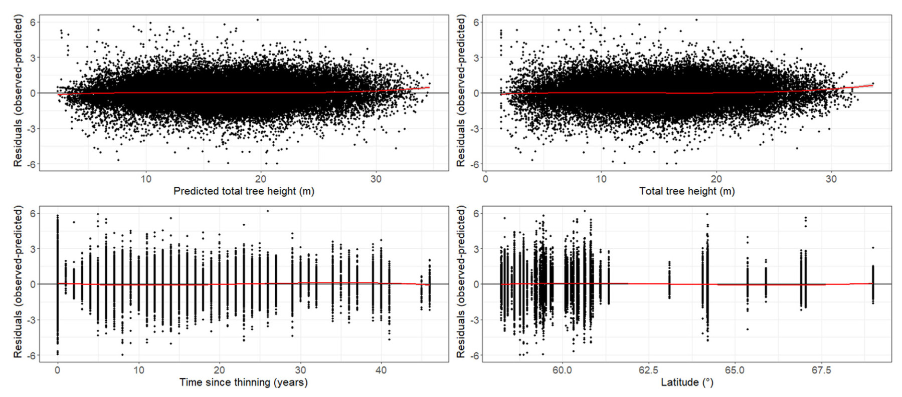
There was no obvious bias when plotting the residuals of ΔHT ƒBASE (Supplementary Material Fig. S3) and ƒFULL over TST and any other explanatory variable or environmental factor (Fig. 4).
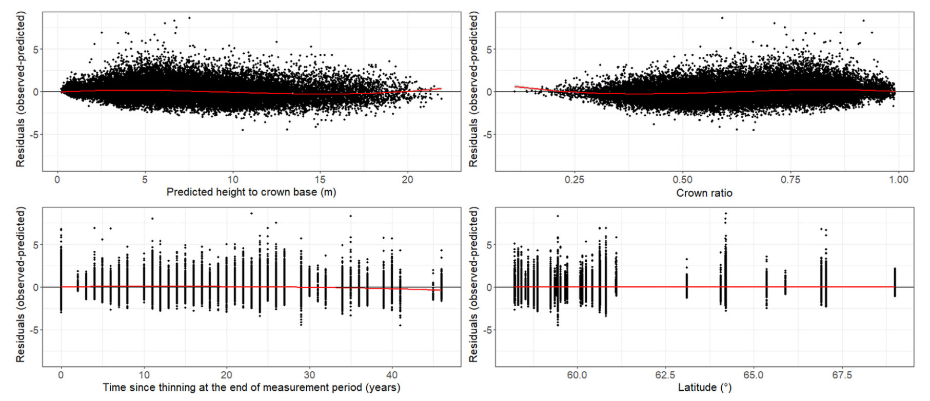
The final ΔHCB ƒBASE included CR, HT, BA, and SI as explanatory variables. Fitting complex thinning modifier as in Eqs. 2-4 did not result in biologically plausible outcomes. However, an indicator variable representing the first eight years after thinning (TST1‒8 = −0.113047) was significant and slightly improved prediction accuracy for trees from non-thinned and thinned stands (data not shown). Adding a modifier following Eq. 5 produced the best performing ƒFULL of the following form (Table 6 and 7, Fig. 2):
| Parameter | ƒBASE | ƒFULL | |||||||
| Estimate | SE | t-value | p-value | Estimate | SE | t-value | p-value | ||
| β100 | ‒13.105355 | 0.41227 | ‒31.79 | < 0.0001 | ‒14.069693 | 0.41012 | ‒34.31 | < 0.0001 | |
| β101 | ‒14.116111 | 0.52402 | ‒26.94 | < 0.0001 | ‒14.715018 | 0.52439 | ‒28.06 | < 0.0001 | |
| β102 | 21.026061 | 0.76135 | 27.62 | < 0.0001 | 21.727372 | 0.76029 | 28.58 | < 0.0001 | |
| β103 | ‒0.125376 | 0.00883 | ‒14.19 | < 0.0001 | ‒0.132922 | 0.00874 | ‒15.21 | < 0.0001 | |
| β104 | 2.219439 | 0.09363 | 23.70 | < 0.0001 | 2.406412 | 0.09372 | 25.68 | < 0.0001 | |
| β105 | ‒0.013652 | 0.00168 | ‒8.12 | < 0.0001 | ‒0.014370 | 0.00176 | ‒8.16 | < 0.0001 | |
| β106 | ‒22.472110 | 1.90811 | ‒11.78 | < 0.0001 | ‒9.986964 | 1.94877 | ‒5.12 | < 0.0001 | |
| β107 | 0.065518 | 0.00463 | 14.16 | < 0.0001 | 0.075643 | 0.00455 | 16.63 | < 0.0001 | |
| β108 | 2.659178 | 0.31383 | 8.47 | < 0.0001 | |||||
| β109 | 1.385330 | 0.10793 | 12.84 | < 0.0001 | |||||
| β110 | 0.148803 | 0.01227 | 12.13 | < 0.0001 | |||||
DownLoad:
CSV
| Variable | ƒBASE | ƒFULL | |||||
| Non-thinned | Thinned | All | Non-thinned | Thinned | All | ||
| ME | 0.0555 | ‒0.0250 | ‒0.0054 | 0.0221 | ‒0.0154 | ‒0.0063 | |
| MAE | 0.8262 | 0.8894 | 0.8740 | 0.8224 | 0.8818 | 0.8673 | |
| MAE% | 13.6168 | 15.9982 | 15.4195 | 14.0757 | 15.8430 | 15.4135 | |
DownLoad:
CSV
| ΔHCB=exp((β100+b100)+(β101+b101)×CR+β102×√CR+(β103+b103)×HT +β104× ln(HT)+β105×BA+β106/BA+β107×SI) ×(1−(β108×(BAREMBABEFORE)β109×exp(−β110×TST))) | (10) |
There was no obvious major bias when plotting the residuals of ΔHCB ƒBASE (Supplementary Material Fig. S4) and ƒFULL over the explanatory variables and other environmental factors (Fig. 5).
This study developed dynamic growth models to predict various individual tree attributes from periodic measurements in non-thinned and thinned Norway spruce stands in Norway. Irrespective of the attribute examined, baseline models without thinning treatment related predictors performed well showing no bias over time since thinning (TST). However, adding thinning related variables either as simple indicator variables for diameter increment (ΔDBH) or multiplicative thinning modifiers (response functions) for height increment (ΔHT) and height to crown base increment (ΔHCB) slightly improved overall prediction accuracy when compared to the corresponding baseline models. Sophisticated modifiers that predict a rapid increase, an early peak, and gradual decline of the thinning effect could not be fitted here.
Multiplicative treatment modifiers are the preferred approach to predict treatment responses because they are potentially the most accurate and detailed way of modelling silvicultural treatment effects including thinning. Multiplicative thinning modifiers as in Eqs. 2-6 do not alter the corresponding baseline model but rather function as modifiers that adjust the outcome of the baseline model in a proportional manner. The resulting relative effect of the modelled treatment response is independent of the baseline equation and thus constant but depends on the outcome of the baseline function in absolute terms. If deemed appropriate, thinning response functions thus can be used in other, separate applications individually, i.e. independent from the corresponding co-developed baseline model.
Continuous and biologically plausible modifiers that predict no effect at the time of thinning, a swift increase followed by an early maximum before the effect gradually declines and becomes zero again, could not be fitted in our study (Kuehne et al., 2016). The modified thinning response function after Liu et al. (1995) fitted to ΔHT somewhat followed the outline response curve but depicted a more symmetrical trajectory over TST. Further, the modelled response effect further needs to be retained after 32 years as it does not approach zero with increasing TST. We believe the experienced difficulties in fitting dynamic modifiers in our study were a result of the periodic data used with its varying multi-year growth intervals that likely concealed the subtle growth differences between trees of non-thinned and thinned stands after accounting for stand density. Previous similar studies that were able to fit such sophisticated modifiers as outlined above either used annual measurements (Kuehne et al., 2016) or short growth intervals of constant, fixed time periods (Liu et al., 1995; Gyawali and Burkhart. 2015).
The final, best performing multiplicative modifiers fitted to our ΔHT and ΔHCB baseline models including an exponentially decreasing thinning effect after a maximum right after thinning for ΔHCB (Hann et al., 2003) seem to be reasonable for ΔHCB and not unlikely for ΔHT. The ideal, i.e. most realistic modifier for ΔHT, however, would potentially depict a delay in the thinning effect of one year because of the partial predefinition of height growth in the growing season prior to thinning. Based on our findings, a basal area removal of 20% would reduce ΔHT and ΔHCB by approximately 5% and 29% approximately nine years after thinning and in the first year following thinning, respectively. Comparable (maximum) values have been reported in similar studies (Liu et al., 1995; Hann et al., 2003; Mäkinen et al., 2006; Kuehne et al., 2016). According to Weiskittel et al. (2011), thinning can either reduce, maintain, or increase tree height growth and the varying behavior is driven by species, crown class, age, and stand density prior to thinning. Our mixed results for ΔHT with indicator variables for various time periods after thinning often signaling a minor increase in ΔHT seem to corroborate this. Insensitivity of ΔHT to thinning has been reported in several previous works (Hynynen, 1995; Westfall and Burkhart, 2001; Hann et al., 2003; Mäkinen and Isomäki, 2004). Given the rather small magnitude and the very short duration, Sharma et al. (2006) and Gyawali and Burkhart (2015) concluded that the thinning induced changes in (dominant) ΔHT observed in their studies were neglectable. Such a conclusion also seems reasonable for our study. A potential decrease in ΔHT and ΔHCB is likely triggered by a reallocation of resources with lateral crown expansion favored over leader growth. In addition, parts if not the entire crown need to adjust to a significantly altered light regime causing a thinning shock to formerly, i.e. pre-thinning shaded foliage.
Although multiplicative response functions could not be fitted for ΔDBH in this study, the indicator variables for TST that were successfully incorporated into the final ΔDBH full model still are proportional and multiplicative in nature. This is a result of the exponential model form used to analyze and predict ΔDBH. TST3, TST4‒5, and TST6‒7 of the full ΔDBH model predict an annual increase in ΔDBH by 40%, 12%, and 8%, respectively, for a thinning intervention removing 20% of pre-treatment basal area. The general magnitude of the modelled ΔDBH thinning effect of our study thus appears to be approximately in line with results from previous similar works (Hynynen, 1995; Jonsson, 1995; Hann et al., 2003; Kuehne et al., 2016). However, the thinning treatment effect usually lasted longer, i.e. up to 15–25 years, in these other studies while a similar delay of the thinning response as found here was reported previously (Thorpe et al., 2007; Mehtätalo et al., 2014). Such a delay is likely to be caused by physiological acclimation to the altered post-thinning growing conditions and the associated resource allocation to root and shoot growth.
Irrespective of the attribute studied here, the residuals of all baseline models without a thinning modifier or thinning indicator variables, respectively, showed no obvious bias when plotted over TST. This was in part to be expected as the main effect of a thinning intervention, i.e. the reduction in stand density is accounted for in each of the baseline models developed here (Weiskittel et al., 2011). All baseline models of this study include at least one metric of competition, i.e. basal area (BA) and/or basal area in larger trees (BAL), representing site occupation and/or stand density. Consequently, a reduction in stand density as a result of a thinning is automatically reflected in the baseline model input variables through altered competition values. Various studies at the stand- as well as the individual tree-level thus found no need to incorporate thinning modifiers into dynamic growth models (Hynynen, 1995; Barrio Anta et al., 2006). However, whether baseline models accurately predict growth of non-thinned as well as thinned stands and trees thereof appears to depend on the kind of forest or species and attribute examined (Weiskittel et al., 2011).
Thinning modifiers or indicator variables representing certain time periods after thinning as in this study still have been examined and successfully added to ΔDBH and stand-level basal area increment baseline equations (Bailey and Ware, 1983; Amateis et al., 1989; de Souza et al., 2022) because of additional, minor effects other than stand density reduction associated with thinning activities (Weiskittel et al., 2011). Among them, fertilization and selection effects appear to be most influential (Hynynen, 1995). Decomposition of organic material including logging slash is often accelerated as a more open canopy following thinning results in a more favorable microclimate on the ground leading to a greater nutrient supply for a limited time. In soil moisture limited forest ecosystems, thinnings also have the potential to improve water availability for residual trees. Further, conventional thinning interventions aim to remove unhealthy, damaged, and thus less vigorous trees. Residual trees not only grew at higher rates before thinning but are also able to better respond to the modified post-thinning growing conditions.
Likely because the baseline models derived in our study are able to capture the main thinning effect, i.e. the reduction in stand density, improvement in model prediction accuracy was mostly rather marginal when extending the models by adding treatment related predictors irrespective of the attribute and approach, which is in agreement with previous studies (Kuehne et al., 2016). While marginal on an annual basis, improvements in prediction accuracy are likely to sum and scale up for longer-term simulation runs of several decades – particularly at the stand level (Kuehne et al., 2016). Still, predictions of our baseline models appear to be reliable because we found no obvious major bias when plotting residuals over TST or any other potentially influential factor. This suggests that complex treatment response functions might not be needed for certain conditions or species, which highlights the often complex and highly varied nature of tree growth following thinning (e.g. Bose et al., 2018).
We thus conclude that i) analyzing periodic growth data of varying multi-year measurement intervals using an annualization method proved to be successful in the detection and quantification of thinning effects not captured in the modification of competition variables and ii) sophisticated, continuous thinning modifiers as initially aimed for here may not be necessary to predict these other individual tree growth-altering thinning effects and thus to build reliable models.
CK: Data curation; Methodology; Formal analysis; Writing - original draft. ARW: Formal analysis; Writing - review & editing. AG: Project administration; Funding acquisition; Writing - review & editing.
The authors declare that they have no known competing financial interests or personal relationships that could have appeared to influence the work reported in this paper.
The authors are indebted to the many people who have been involved in the installment and monitoring of the permanent sample plots analyzed in this work. We also like to thank the reviewer for constructive comments on the previous version of this paper and the associate editor for handling the manuscript.
Supplementary data to this article can be found online at https://doi.org/10.1016/j.fecs.2022.100060.
Figures(5) / Tables(7)


Supported by: Beijing Renhe Information Technology Co. Ltd. Technical support: info@rhhz.net
| Attribute | Non-thinned | Thinned | All | ||||||||||||
| Mean | SD | Min | Max | Mean | SD | Min | Max | Mean | SD | Min | Max | ||||
| ΔDBH | |||||||||||||||
| DBH (cm) | 13.30 | 5.68 | 1.00 | 43.10 | 15.81 | 6.09 | 1.50 | 44.70 | 14.91 | 6.07 | 1.00 | 44.70 | |||
| HT (m) | 12.98 | 5.27 | 1.30 | 33.60 | 13.66 | 5.06 | 1.60 | 35.10 | 13.42 | 5.15 | 1.30 | 35.10 | |||
| HCB (m) | 5.66 | 3.94 | 0 | 20.50 | 4.38 | 3.33 | 0.10 | 22.39 | 4.84 | 3.61 | 0 | 22.39 | |||
| CR (m·m−1) | 0.61 | 0.18 | 0.04 | 1.00 | 0.72 | 0.14 | 0.02 | 0.99 | 0.68 | 0.16 | 0.02 | 1.00 | |||
| BAL (m2·ha−1) | 24.44 | 15.27 | 0 | 85.64 | 16.93 | 10.95 | 0 | 63.44 | 19.62 | 13.17 | 0 | 85.64 | |||
| BA (m2·ha−1) | 39.08 | 15.57 | 2.96 | 86.58 | 28.23 | 11.40 | 6.33 | 63.82 | 32.12 | 14.05 | 2.96 | 86.58 | |||
| SI (m) | 15.57 | 4.45 | 6.64 | 28.61 | 15.45 | 2.80 | 10.10 | 21.80 | 15.49 | 3.48 | 6.64 | 28.61 | |||
| ΔHT | |||||||||||||||
| DBH (cm) | 15.01 | 6.58 | 1.00 | 43.10 | 17.95 | 6.57 | 1.50 | 44.70 | 17.02 | 6.72 | 1.00 | 44.70 | |||
| HT (m) | 13.58 | 5.76 | 1.30 | 33.60 | 14.82 | 5.23 | 1.60 | 31.70 | 14.42 | 5.43 | 1.30 | 33.60 | |||
| HCB (m) | 5.59 | 4.23 | 0.01 | 20.50 | 4.88 | 3.74 | 0.10 | 21.00 | 5.10 | 3.91 | 0.01 | 21.00 | |||
| CR (m·m−1) | 0.64 | 0.20 | 0.11 | 0.99 | 0.70 | 0.15 | 0.16 | 0.99 | 0.68 | 0.17 | 0.11 | 0.99 | |||
| BAL (m2·ha−1) | 20.34 | 16.33 | 0 | 85.64 | 15.24 | 12.12 | 0 | 63.44 | 16.85 | 13.80 | 0 | 85.64 | |||
| BA (m2·ha−1) | 39.11 | 16.64 | 2.96 | 86.58 | 30.12 | 11.37 | 6.33 | 63.82 | 32.97 | 13.91 | 2.96 | 86.58 | |||
| SI (m) | 15.91 | 4.08 | 6.64 | 28.61 | 15.54 | 2.88 | 10.10 | 21.80 | 15.66 | 3.31 | 6.64 | 28.61 | |||
| ΔHCB | |||||||||||||||
| DBH (cm) | 16.08 | 6.53 | 2.30 | 43.10 | 18.28 | 6.43 | 2.40 | 44.70 | 17.75 | 6.52 | 2.30 | 44.70 | |||
| HT (m) | 14.63 | 5.60 | 2.30 | 32.00 | 15.11 | 5.06 | 2.20 | 31.70 | 14.99 | 5.20 | 2.20 | 32.00 | |||
| HCB (m) | 6.45 | 4.05 | 0.10 | 20.50 | 5.08 | 3.68 | 0.10 | 21.00 | 5.41 | 3.82 | 0.10 | 21.00 | |||
| CR (m·m−1) | 0.59 | 0.17 | 0.11 | 0.99 | 0.69 | 0.15 | 0.16 | 0.99 | 0.67 | 0.16 | 0.11 | 0.99 | |||
| BAL (m2·ha−1) | 22.40 | 17.05 | 0 | 74.74 | 15.58 | 12.00 | 0 | 63.44 | 17.24 | 13.72 | 0 | 74.74 | |||
| BA (m2·ha−1) | 44.12 | 14.26 | 10.52 | 74.99 | 30.78 | 10.66 | 8.48 | 63.82 | 34.02 | 12.97 | 8.48 | 74.99 | |||
| SI (m) | 14.94 | 4.55 | 6.64 | 23.27 | 15.31 | 2.96 | 10.10 | 21.80 | 15.22 | 3.42 | 6.64 | 23.27 | |||
DownLoad:
CSV
| Parameter | ƒBASE | ƒFULL | |||||||
| Estimate | SE | t-value | p-value | Estimate | SE | t-value | p-value | ||
| β80 | ‒5.047643 | 0.10520 | ‒47.98 | < 0.0001 | ‒5.468100 | 0.10565 | ‒51.76 | < 0.0001 | |
| β81 | ‒0.039723 | 0.00379 | ‒10.47 | < 0.0001 | ‒0.038439 | 0.00392 | ‒9.80 | < 0.0001 | |
| β82 | 0.875792 | 0.01267 | 69.12 | < 0.0001 | 0.778875 | 0.01286 | 60.55 | < 0.0001 | |
| β83 | 0.903008 | 0.01660 | 54.39 | < 0.0001 | 1.023460 | 0.01678 | 60.98 | < 0.0001 | |
| β84 | ‒0.000668 | 0.00001 | ‒137.06 | < 0.0001 | ‒0.000695 | 0.00001 | ‒139.51 | < 0.0001 | |
| β85 | ‒0.308305 | 0.00733 | ‒42.05 | < 0.0001 | ‒0.122793 | 0.00851 | ‒14.43 | < 0.0001 | |
| β86 | 1.028367 | 0.01953 | 52.67 | < 0.0001 | 0.999885 | 0.01944 | 51.43 | < 0.0001 | |
| β87 | 1.692007 | 0.05448 | 31.06 | < 0.0001 | |||||
| β88 | 0.555523 | 0.06355 | 8.74 | < 0.0001 | |||||
| β89 | 0.405501 | 0.05523 | 7.34 | < 0.0001 | |||||
DownLoad:
CSV
| Variable | ƒBASE | ƒFULL | |||||
| Non-thinned | Thinned | All | Non-thinned | Thinned | All | ||
| ME | ‒0.0013 | 0.0029 | 0.0014 | 0.0201 | ‒0.0082 | 0.0020 | |
| MAE | 0.4310 | 0.5332 | 0.4965 | 0.4319 | 0.5270 | 0.4929 | |
| MAE% | 3.2616 | 3.2330 | 3.2432 | 3.2746 | 3.1966 | 3.2246 | |
DownLoad:
CSV
| Parameter | ƒBASE | ƒFULL | |||||||
| Estimate | SE | t-value | p-value | Estimate | SE | t-value | p-value | ||
| β90 | ‒3.817176 | 0.13148 | ‒29.03 | < 0.0001 | ‒3.899612 | 0.13273 | ‒29.38 | < 0.0001 | |
| β91 | ‒0.034339 | 0.00437 | ‒7.85 | < 0.0001 | ‒0.037829 | 0.00445 | ‒8.50 | < 0.0001 | |
| β92 | 0.629971 | 0.02395 | 26.31 | < 0.0001 | 0.685842 | 0.02473 | 27.74 | < 0.0001 | |
| β93 | 0.546126 | 0.02114 | 25.84 | < 0.0001 | 0.584605 | 0.02139 | 27.33 | < 0.0001 | |
| β94 | ‒0.000365 | 0.00003 | ‒12.05 | < 0.0001 | ‒0.000358 | 0.00003 | ‒12.00 | < 0.0001 | |
| β95 | 0.460302 | 0.03296 | 13.97 | < 0.0001 | 0.446552 | 0.03301 | 13.53 | < 0.0001 | |
| β96 | ‒1.387400 | 0.17136 | ‒8.10 | < 0.0001 | |||||
| β97 | 28.684904 | 1.93656 | 14.81 | < 0.0001 | |||||
DownLoad:
CSV
| Variable | ƒBASE | ƒFULL | |||||
| Non-thinned | Thinned | All | Non-thinned | Thinned | All | ||
| ME | 0.0570 | ‒0.0293 | −0.0019 | 0.0436 | ‒0.0248 | −0.0031 | |
| MAE | 0.5918 | 0.5969 | 0.5953 | 0.5899 | 0.5966 | 0.5945 | |
| MAE% | 4.3839 | 3.8268 | 4.0034 | 4.3682 | 3.8229 | 3.9958 | |
DownLoad:
CSV
| Parameter | ƒBASE | ƒFULL | |||||||
| Estimate | SE | t-value | p-value | Estimate | SE | t-value | p-value | ||
| β100 | ‒13.105355 | 0.41227 | ‒31.79 | < 0.0001 | ‒14.069693 | 0.41012 | ‒34.31 | < 0.0001 | |
| β101 | ‒14.116111 | 0.52402 | ‒26.94 | < 0.0001 | ‒14.715018 | 0.52439 | ‒28.06 | < 0.0001 | |
| β102 | 21.026061 | 0.76135 | 27.62 | < 0.0001 | 21.727372 | 0.76029 | 28.58 | < 0.0001 | |
| β103 | ‒0.125376 | 0.00883 | ‒14.19 | < 0.0001 | ‒0.132922 | 0.00874 | ‒15.21 | < 0.0001 | |
| β104 | 2.219439 | 0.09363 | 23.70 | < 0.0001 | 2.406412 | 0.09372 | 25.68 | < 0.0001 | |
| β105 | ‒0.013652 | 0.00168 | ‒8.12 | < 0.0001 | ‒0.014370 | 0.00176 | ‒8.16 | < 0.0001 | |
| β106 | ‒22.472110 | 1.90811 | ‒11.78 | < 0.0001 | ‒9.986964 | 1.94877 | ‒5.12 | < 0.0001 | |
| β107 | 0.065518 | 0.00463 | 14.16 | < 0.0001 | 0.075643 | 0.00455 | 16.63 | < 0.0001 | |
| β108 | 2.659178 | 0.31383 | 8.47 | < 0.0001 | |||||
| β109 | 1.385330 | 0.10793 | 12.84 | < 0.0001 | |||||
| β110 | 0.148803 | 0.01227 | 12.13 | < 0.0001 | |||||
DownLoad:
CSV
| Variable | ƒBASE | ƒFULL | |||||
| Non-thinned | Thinned | All | Non-thinned | Thinned | All | ||
| ME | 0.0555 | ‒0.0250 | ‒0.0054 | 0.0221 | ‒0.0154 | ‒0.0063 | |
| MAE | 0.8262 | 0.8894 | 0.8740 | 0.8224 | 0.8818 | 0.8673 | |
| MAE% | 13.6168 | 15.9982 | 15.4195 | 14.0757 | 15.8430 | 15.4135 | |
DownLoad:
CSV

 Email Alerts
 RSS Feeds